Contingency tables and Correspondence analysis

1. Contingency tables and Correspondence analysis • Contingency table • Pearson’s chi-squared test for association • Correspondence analysis • Plots • References • Exercises

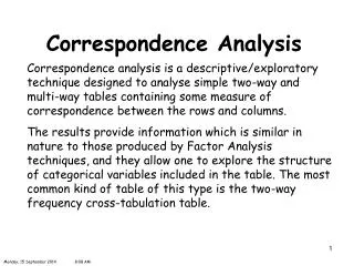
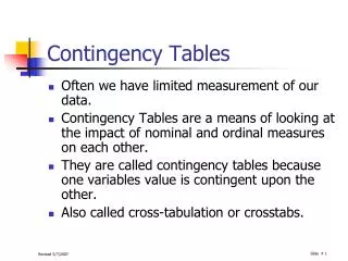
2. Contingency tables Contingency tables are often used in social sciences (such as sociology, education, psychology). These tables can be considered as frequency tables. Rows and columns are some categorical variables. If variables are continuous then we can use bins for these continuous variables and convert them to categorical variables. Categorical variables have discrete values. For example eye colours: Light, blue, medium, dark. Contingency tables sometimes are called as incidence matrices also. Example of contingency tables. Eye and hair colours of schoolchildren from Caitness in Scotland. There are 5387 schoolchildren divided by hair and eye colours. There are 5 hair and 4 eye colours. fair red medium dark black blue 326 38 241 110 3 light 688 116 584 188 4 medium 343 84 909 412 26 dark 98 48 403 681 85 First question is if there is association between columns and rows. If there is some association then we want to find some structure in this data table. I.e. which columns might be related with which rows. First question is answered by Pearson chi-squared test and the second one is approached by the correspondence analysis.

3. Pearson chi-squared test Suppose that we have a data matrix N that has I rows and J columns. Elements of the matrix are nij. Let us use the following notations: Then Pearson chi-squared statistic for testing the null-hypothesis no row-column association is calculated: with degrees of freedom (I-1)(J-1=IJ-(I+J-1). If the value of this statistic is high then we can say that there is row-column association. If the value of this statistic is low then we can say that there is no row-column association. For above example chi-squared test carried out in R gives: --------------------------------------------------------------- Pearson's Chi-squared test data: caith X-squared = 1240.039, df = 12, p-value = < 2.2e-16 --------------------------------------------------------------- This test shows that null-hypothesis should rejected. I.e. there is strong evidence there is row-column association. This result could be expected.

4. Contingency tables: homogeneity and heterogeneity t=X2/n is the coefficient of association called as Pearson’s mean-square contingency. It is now called the total inertia. The total inertial is measure of homogeneity/heterogeneity of the table. If t is large it is measure of heterogeneity and if t is small it is measure of homogeneity of the table. Homogeneity means that there is no row-column association. t can also be calculated using: Second summation is sum of a weighted squared distance between the vector of relative frequency of the ith row (i.e. jth row profile – pij/ri) and the average row profile – c. Inverse of the elements of c are the weights. It is known as chi-squared distance between ith row profile and the average row profile.The total inertia is is further weighted sums of I chi-squared distances. The weights are the elements of r. If all elements of row profiles are close to the average row profile then table is homogenous. Otherwise table is heterogeneous. We can do similar calculations for the column profiles. It is done easily by changing roles of r and c. This distances are similar to Euclidean distances and techniques used for Euclidean distances can also be used for this case. We will learn techniques for metric scaling in one of the future lectures.

5. Contingency table: Correspondence analysis Usual techniques for contingency table analysis is the correspondence analysis. Its aim is to try to find some association between rows and columns. It should of course be carried out if chi-squared test shows that there might be row column associations. Let us use the following notations: P is matrix of the element pij. Then r and c can be defined as: Where 1 is corresponding dimensional column vector. I.e. if c is calculated then its dimension is I and if r is calculated its dimension is J. Let us further define diagonal matrices formed by r and c: Let matrix E be: We can see that elements of E have been used above to calculated chi-squared distances, the total inertia etc. Elements of E are related with standardised Pearsonian residuals. These residuals are elements that contribute to calculation of X2 statistic.

6. Contingency table and SVD Now we can use SVD of E to analyse the contingency table. SVD of E is: Where U and V are the orthogonal matrices containing eigenvectors of EET and ETE correspondingly. D is the diagonal matrix containing square roots of non-zero eigenvalues of the matrices - EET and ETE. D is also called the canonical correlation. Row profiles are calculated using: Rows of this matrix are row profiles. Column profiles are calculated using: Pairs of rows of F and G are the elements of the orthogonal decomposition of the residuals in a decreasing order. This approach is called the correspondence analysis of the contingency table. Centroids of F and G are 0. F and G are related:

7. Correspondence analysis Elements of D are called the principal inertias. They are also related to the canonical correlations given by the package R. Larger value of D means that the corresponding element has higher importance. It is usual to use one or two elements of F and G. Then these elements are used for various plots. For pictorial representation either columns and row are plotted in and ordered form or biplots is used to find possible association between rows and columns. Let us use the example caith from the R package and analyse it. As it was mentioned there are some association between the rows and the columns (chi-squared was very large number).

8. Plot of correspondence analysis: Example This is pictorial form of the table itself. Positions of rows and columns correspond to row and column scores. This picture already can tell something about the structure of the data.

9. Biplot for the correspondence analysis Biplot produced by R: Black are rows and red are columns. Position of the points correspond to their scores. Again from this picture we can deduce some structure about data.

10. R commands for contingency tables and correspondence analysis For correspondence analysis we need libraries ctest, MASS and mva. We need to load them library(mva) library(MASS) library(ctest) To perform chi-squared test we can use (load data first) data(caith) chisq.test(caith) If there is some association between rows and columns then we can start usinng the correspondence analysis: ccaith = corresp(caith,nf=1) nf is the number of factors we want to find. we can plot this using the plot command plot(ccaith) – If we have only 1 factor then result will be pictorial representation of the table. if nf=2 then result will be the biplot.

11. References • Krzanowski WJ and Marriout FHC. (1994) Multivatiate analysis. Vol 2. Kendall’s library of statistics

12. Exercises 5 a) Take the data from R. Data set is deaths – monthly death rates from lung deceases in the UK. These data cannot be used directly for chisq.test and corresp commands. Data should be converted to data matrix. It can be done using data(deaths) dth = matrix(deaths,ncol=12,byrow=TRUE) Now try to analyse these data using corresponding analysis technique b) Take data set accdeaths (accidental deaths in the USA from 1973-1978). These data should also be converted to data matrix. If you are curious try drivers and analyse it. This is data set on drivers deaths. You might see an interesting feature.