Contingency Table and Correspondence Analysis
Contingency Table and Correspondence Analysis. Nishith Kumar Department of Statistics BSMRSTU. and. Mohammed Nasser Department of Statistics RU. Overview. Contingency table. Some real world problem for contingency table Pearson chi-squared test

Contingency Table and Correspondence Analysis
E N D
Presentation Transcript
Contingency Table and Correspondence Analysis Nishith Kumar Department of Statistics BSMRSTU and Mohammed Nasser Department of Statistics RU
Overview • Contingency table. • Some real world problem for contingency table • Pearson chi-squared test • Probabilistic interpretation of matrices • Contingency tables: Homogeneity and Heterogeneity • Historical background of correspondence analysis • Correspondence analysis (CA) • Correspondence analysis and eigenvalues. • Singular value decomposition. • Calculation procedure of CA • Interpretation of correspondence analysis • R code and examples • Conclusion
Contingency Table In statistics, a contingency table (also referred to as cross tabulation or cross tab) is a type of table in a matrix format that displays the (multivariate) frequency distribution of the variables. The term contingency table was first used by Karl Pearson in 1904. Sometimes contingency table is called incidence matrix. Contingency tables are often used in social sciences (such as sociology, education, psychology). These tables can be considered as frequency tables. Rows and columns are some categorical variables. If variables are continuous then we can use bins for these continuous variables and convert them into categorical ones.
Real Problem Cross-tabulation of age groups by perceived health status 1. Is there any relation between different age group and perceived health status? 2. How can you visualize this type of relationship? 3. How can you find the similarity of row category? 4. How can you Interprete – distances between categories of row and columnvariables
Real Problem Suppose we have the following contingency table 1. How can we analyze contingency table type data? 2. How can we converts frequency table data into graphical displays. 3. How can we find the similarity of column category? 4. How can we find the similarity of row category? 5. How can we find the relationship of row and column category simultaneously?
Real Problem Survey of effects of four different drug types. Patients gave score for each drug type (excellent, very good, good, fair, poor). Number of all elements is 121. excellent very good good fair poor Drug A 6 8 10 1 5 Drug B 12 8 3 3 5 Drug C 0 3 12 6 10 Drug D 1 1 8 12 7 • Is there is association between columns and rows? • If there is some association then how can we find some structure in this data table? • Can we order columns and rows by their closeness? • Can we find associations between columns and rows?
Pearson chi-squared test Suppose that we have a data matrix X that has I rows and J columns. Elements of the matrix are xij. Let us use the following notations: r and c are row and column sums, R and C are row and column profiles, respectively. Q is difference between P and product of row and column sums.
Pearson chi-squared test (Cont.) More notations and relations: Row and column inertias are multiple of chi-squared with degrees of freedom (I-1)(J-1). Multiplicity is 1/n. If P would be probability then if there would be no association between rows and columns then Q would be 0. It is equivalent to saying that rows and columns are independent
Pearson chi-squared test (Cont.) For Smoke Data: R Code: library(ca) library(MASS) ca(smoke) chisq.test(smoke) Principal inertias: 1 2 3 Value 0.074759 0.010017 0.000414 Percentage 87.76% 11.76% 0.49% Rows: SM JM SE JE SC Inertia 0.002673 0.011881 0.038314 0.026269 0.006053 Columns: none light medium heavy Inertia 0.049186 0.007059 0.012610 0.016335 We have seen, Chi square value = total Inertia * Grand total, df= (no. of row - 1 ) * (no. of Column -1) Chi squared = 16.4416, df = 12, p-value = 0.1718
Pearson chi-squared test (Cont.) Drag Data R Code: library(ca) library(MASS) ca(drug) chisq.test(drug)) Principal inertias : 1 2 3 inertias 0.304667 0.077342 0.007015 Percentage 78.32% 19.88% 1.8% Rows: Drug A Drug B Drug C Drug D Inertia 0.055280 0.143372 0.071340 0.119030 Columns: excellent verygood good fair poor Inertia 0.152430 0.060843 0.044719 0.111385 0.019646 Chi square value = total Inertia * Grand total, df= (no. of row - 1 ) * (no. of Column -1) Chi squared = 47.0718, df = 12, p-value = 4.53e-06 I.e. there is strong evidence that there is row-column association.
Pearson chi-squared test (Cont.) Health Data: R Code: library(ca) library(MASS) ca(health) chisq.test(health)) Principal inertias: 1 2 3 4 Value 0.136603 0.00209 0.001292 0.000474 Percentage 97.25% 1.49% 0.92% 0.34% Rows: 16-24 25-34 35-44 45-54 55-64 65-74 75+ Inertia 0.027020 0.021316 0.006900 0.001667 0.022711 0.033288 0.027557 Columns: VG GOOD REG BAD VB Inertia 0.024279 0.022368 0.045823 0.037955 0.010034 Chi square value = total Inertia * Grand total, df= (no. of row - 1 ) * (no. of Column -1) Chi squared = 894.8607, df = 24, p-value < 2.2e-16 I.e. there is strong evidence that there is row-column association.
Probabilistic Interpretation of Matrices , If the matrixPwould be a probability matrix i.e. each element pij are probability of happening rows and columns simultaneously then we can have the following interpretation of the involved matrices: • Elements of r are the marginal probabilities of rows. Elements of c are the marginal probabilities of columns. • Elements of Q are differences between joint probability and product of individual probabilities. In some sense this matrix represents the degree of dependencies of rows and columns • Elements of R are the conditional probabilities of columns when row is known • Elements of C are the conditional probabilities of rows when column is known • Total inertia is the total indicator of dependencies of rows and columns.
Marginal probability of Drag Data X • Elements of r are the marginal probabilities of columns. Elements of c are the marginal probabilities of rows
Degree of dependencies of rows and columns • Elements of Q are differences between joint probability and product of individual probabilities. In some sense this matrix represents the degree of dependencies of rows and columns Q excellent very good good fair poor Drug A 0.01065501 0.02513490 0.0150262960 -0.036814425 -0.014001776 Drug B 0.05894406 0.02376887 -0.0450788881 -0.021788129 -0.015845912 Drug C -0.04022949 -0.01755345 0.0293012772 0.003005259 0.025476402 Drug D -0.02936958 -0.03135032 0.0007513148 0.055597295 0.004371286 See slide no. 19 for R code
Conditional Probabilities and Inertias 3) Elements of R are the conditional probabilities of columns when row is known R excellent very good good fair poor Drug A 0.20000000 0.26666667 0.33333333 0.03333333 0.1666667 Drug B 0.38709677 0.25806452 0.09677419 0.09677419 0.1612903 Drug C 0.00000000 0.09677419 0.38709677 0.19354839 0.3225806 Drug D 0.03448276 0.03448276 0.27586207 0.41379310 0.2413793 4) Elements of C are the conditional probabilities of rows when column is known C DrugA DrugB Drug CDrugD Excellent 0.31578947 0.63157895 0.0000000 0.05263158 Very good 0.40000000 0.40000000 0.1500000 0.05000000 good 0.30303030 0.09090909 0.3636364 0.24242424 Fair 0.04545455 0.13636364 0.2727273 0.54545455 poor 0.18518519 0.18518519 0.3703704 0.25925926 • Total inertia is the total indicator of dependencies of rows and columns. • Small inertia indicate there is no row column association.
Similarly we can find the following measurement for Smoke data and Health Status data. • Marginal probabilities , • Degree of dependencies of row and column • Conditional probabilities • Inertias
Contingency Tables: Homogeneity and Heterogeneity t=in(I)=in(J)=X2/n is the coefficient of association called as Pearson’s mean-square contingency. It is the total inertia. The total inertia is a measure of homogeneity/heterogeneity of the table. If t is large it is a measure of heterogeneity and if t is small it is a measure of homogeneity of the table. Homogeneity means that there is no row-column association. t can also be calculated using:
Contingency Tables: Homogeneity and Heterogeneity( Cont.) We can interpret the following formula by the following way • Second summation is sum of a weighted squared distance between the vector of relative frequency of the ith row (i.e. jth row profile – pij/ri) and the average row profile – c. Inverse of the elements of c are the weights. • It is known as chi-squared distance between ith row profile and the average row profile. • The total inertia is further weighted sums of I chi-squared distances. • The weights are the elements of r. • If all elements of row profiles are close to the average row profile then table is homogenous. Otherwise table is heterogeneous. We can do similar calculations for the column profiles. It is done easily by changing roles of r and c.
Calculations of Inertia to Find Out the Homogeneity or Heterogeneity We can calculate t by R from the following code, library(ca) library(MASS) ######Read Data######## ###### Probability Matrix####### pdrag<-drug/121 c<-colSums(pdrag) r<-rowSums(pdrag) Dr<-diag(r) Dc<-diag(c) q<-pdrag-r%*%t(c) R<-ginv(Dr)%*%as.matrix(pdrag) C<-ginv(Dc)%*%t(as.matrix(pdrag)) sp<-0 tsp<-0 t<-0 for(i in 1:4){ for (j in 1:5){ sp[j]<-((((pdrag[i,j]/r[i])-c[j])*((pdrag[i,j]/r[i])-c[j]))/c[j]) } tsp[i]<-colSums(as.matrix(sp)) t[i]<-r[i]*tsp[i] } ti<-colSums(as.matrix(t)) Total inertia for Drug data is t = 0.3890234
Historical Background of Correspondence Analysis The CA solution was shown by (Greenacre 1984) Correspondence analysis (CA) was first proposed by Hirschfeld 1935 Hirschfeld 1935 Later CA was developed by Jean-Paul Benzécri 1973 It is incorporated in R in 2009
Correspondence Analysis Correspondence analysis is a statistical technique used to analyze categorical data (Benzecri, 1992) and provides a graphical representation of cross tabulations or contingency tables. Correspondence analysis (CA) can be viewed as a generalized principal component analysis tailored for the analysis of qualitative data. Although CA was originally created to analyze cross tabulation but CA is so multipurpose that it is used with a lot of other numerical data table types. It is formally applicable to any data matrix with nonnegative entries.
Objectives of CA The main objectives of CA are to transform a dataset into two factor scores (rows and columns) that give the best representation of the similarity structure of the rows and columns of the table. Correspondence analysis is used to reduce the dimension of a data matrix as in principal component analysis. So using CA we can visualize the data two or three dimensionally.
Correspondence analysis and eigenvalues For a given contingency table we calculate row and column profiles. Now we want to find a vector (g) when multiplied by row profiles from the left will have highest possible variance. It means that we want to maximize To make this problem solvable we add an additional constraint (similar to PCA). We want weighted norm of the vector to be unit and weighted mean to be 0. Weights are column sums. So we have to maximize
Correspondence analysis and eigenvalues (cont.) To maximize the function we can use the Lagrange multipliers technique. Thus the Lagrange function Now differentiating L by g and put that equal to zero Thus the problem reduces to the eigenvalue problem. As a result we will have principal coordinates for columns. Similarly we can find principal coordinates for row. This problem easily and compactly solved if we use singular value decomposition.
Singular Value Decomposition X Λ = Row orthonormal containing the eigenvectors of XTX. VT U n×n n×n m×n m×n Real, where (n≤ m) Diagonal matrix, containing the singular values of matrix X. column orthonormal containing the eigenvectors of XXT. • XV=U Λ, The columns U Λindicate the PCs • Left singular vector shows the structure of observations. • Right singular vector shows the structure of variables.
Correspondence Analysis Calculation Procedure To obtain coordinates using SVD, the computational algorithm of the row and column profiles with respect to principle axes are given below X Grand total Diagonal Matrix Row total P r Column Total c Calculate the matrix of standardized residuals [Using SVD] U is a (m×n) column orthonormal matrix (UTU=I), containing the eigenvectors of the symmetric matrix PPT and VT is a (nxn) row orthonormal matrix (VTV=I), containing the eigenvectors of the symmetric matrix PTP. The principal coordinates of rows: The principal coordinates of columns: respectively Standard row and column coordinates are First few (one or two) elements of F and G are usually taken and plotted simultaneously.
Interpretation of Correspondence analysis Elements of Λ are called the principal inertias. They are also related to the canonical correlations given by the package R. Larger value of Λ means that the corresponding element has higher importance. It is usual to use one or two elements of F and G. Then these elements are used for various plots. For pictorial representation either columns or rows are plotted in and ordered form or biplots is used to find possible association between rows and columns as well as their order. Correspondence Analysis can be considered as a dimension reduction technique and can be used together with others (for example PCA). Comparative application of different dimension reduction technique may give insight to the problem and structure in the data.
Algorithm of Correspondence Analysis • Take a contingency table (X) and find sum of all elements (total sum= n) • Divide all elements by the total sum (call it P) • Find row and column sums (r and c) • Calculate the matrix of standardized residuals, • Find generalized SVD of the S. • Find principal row and column coordinates. Take few elements and plot them • Analyze the results (order and closeness of columns and rows, possible associations between columns and rows).
Correspondence Analysis in Drug data R code: drug<- read.table(text = " qlt excellent verygood good fair poor DrugA 6 8 10 1 5 DrugB 12 8 3 3 5 Drugc 0 3 12 6 10 DrugD 1 1 8 12 7 ", row.names = 1, header = TRUE) plot(ca(drug), mass = c(TRUE, TRUE)) plot(ca(drug), mass = c(TRUE, TRUE), arrows = c(FALSE, TRUE)) Summary(ca(drug))
Biplot of Drug data using Correspondence Analysis Principal inertias (eigenvalues): dim value % cum% 1 0.304667 78.3 78.3 2 0.077342 19.9 98.2 3 0.007015 1.8 100.0 -------- ----- Total: 0.389023 100.0
Correspondence analysis in Smoke Data Principal inertias (eigen values): dim value % cum% scree plot 1 0.074759 87.8 87.8 ************************* 2 0.010017 11.8 99.5 *** 3 0.000414 0.5 100.0 library(ca) data("smoke") plot(ca(smoke), mass = c(TRUE, TRUE)) Summary(ca(smoke))
Biplot using Correspondence analysis library(ca) data("smoke") plot(ca(smoke), mass = c(TRUE, TRUE), arrows = c(FALSE, TRUE))
Three Dimensional plot using Correspondence analysis library(ca) data("smoke") plot3d.ca(ca(smoke, nd=3))
Correspondence analysis in Health Data library(ca) health<- read.table(text = " age VG GOOD REG BAD VB 16-24 243 789 167 18 6 25-34 220 809 164 35 6 35-44 147 658 181 41 8 45-54 90 469 236 50 16 55-64 53 414 306 106 30 65-74 44 267 284 98 20 75+ 20 136 157 66 17 ", row.names = 1, header = TRUE) plot(ca(health), mass = c(TRUE, TRUE))
Biplot of Health Data Correspondence analysis library(ca) health<- read.table(text = " age VG GOOD REG BAD VB 16-24 243 789 167 18 6 25-34 220 809 164 35 6 35-44 147 658 181 41 8 45-54 90 469 236 50 16 55-64 53 414 306 106 30 65-74 44 267 284 98 20 75+ 20 136 157 66 17 ", row.names = 1, header = TRUE) plot(ca(health), mass = c(TRUE, TRUE), arrows = c(FALSE, TRUE))
Conclusion • In conclusion we can say that correspondence analysis can • Converts frequency table data into graphical displays • Show the similarity of row category • Show the similarity of column category • Show the relationship of row and column category simultaneously Although CA was originally created to analyze cross tabulation but CA is so multipurpose that it is used with a lot of other numerical data table types. It is formally applicable to any data matrix with nonnegative entries.
Future Studies • Study Multiple correspondence analysis. • High dimensional data analysis using Correspondence Analysis. • Assess the effect of outliers. • The 1st CA axis is reliable, but 2nd and later axes are quadratic distortions of the first – produces the “arch effect”. So my future study is how to solve this problem. • Application of CA in Microarray data to find out the gene pattern and similarity of gene structure. • Missing value and outlier is a general problem in microarray data. So solving missing value and outlier problem my target is to propose a robust correspondence analysis method that can handle both outlier and missing value problem
References • Benzécri, J.-P. (1973). L'Analyse des Données. Volume II. L'Analyse des Correspondances. Paris, France: Dunod. • Greenacre, Michael (1983). Theory and Applications of Correspondence Analysis. London: Academic Press. ISBN 0-12-299050-1 • Greenacre, Michael (2007). Correspondence Analysis in Practice, Second Edition. London: Chapman & Hall/CRC. • Greenacre, M. and Nenadic,O. (2007), “Correspondence Analysis in R, with Two- and Three-dimensional Graphics: The ca Package”,Journal of Statistical Software,Vol-20 ,Issue-30. 5. Hirschfeld, H.O. (1935) "A connection between correlation and contingency", Proc. Cambridge Philosophical Society, 31, 520–524.