Contingency Table Analysis
Contingency Table Analysis. contingency tables show frequencies produced by cross-classifying observations e.g., pottery described simultaneously according to vessel form & surface decoration. most statistical tests for tables are designed for analyzing 2-dimensions

Contingency Table Analysis
E N D
Presentation Transcript
contingency tables show frequencies produced by cross-classifying observations • e.g., pottery described simultaneously according to vessel form & surface decoration
most statistical tests for tables are designed for analyzing 2-dimensions • only examine the interaction of two variables at one time… • most efficient when used with nominal data • using ratio data means recoding data to a lower scale of measurement (ordinal) • means ignoring some of the information originally available…
still, you might do this, particularly if you are interested in association between metric and non-metric variables • e.g.: variation in pot size vs. surface decoration… • may decide to divide pot size into ordinal classes…
small medium large small large
rim diameter: slip: • other options may let you retain more of the original information content
could use a “t-test” to test the equality of the means • makes full use of ratio data… non-specularslip specularslip
because we think there may be some kind of interaction between the variables… • basic question: can the state of one variable be predicted from the state of another variable? • if not, they are independent
expected counts • a baseline to which observed counts can be compared • counts that would occur by random chance ifthe variables are independent, over the long run • for any cell E = (col total * row total)/table total
significance • = probability of getting, by chance, a table as or more deviant than the observed table, if the variables are independent • ‘deviant’ defined in terms of expected table • no causality is necessarily implied by the outcome • but, causality may well be the reason for observed association… • e.g.: grave goods and sex
Fisher’s Exact Test • just for 2 x 2 tables • useful where chi-square test is inappropriate • gives the exact probability of all tables with • the same marginal totals • as or more deviant than the observed table…
P = (a+b)!(a+c)!(b+d)!(c+d)! / (N!a!b!c!d!) P = 5!5!6!6! / 11!4!1!1!5! = 5*6!6! / 11! P = 5*6!6! / 11! = 5*6! / 11*10*9*8*7 P = 5*6! / 11*10*9*8*7 = 3600 / 55440 P = .065
P = .065 use R (or Excel) if the counts aren’t too large… > fisher.test(x)
(observed) (expected) 0.013 0.325 • P = 0.065+0.002 = 0.067 or • P = 0.067+0.013 = 0.080 0.162 0.065 0.433 0.002
in R: > fisher.test(x, alt = "two.sided") > fisher.test(x, alt = “greater”) [i.e.: H1: odds ratio > 1] • 2-tailed test = 0.067+0.013 = 0.080 • 1-tailed test = 0.065+0.002 = 0.067
Chi-square Statistic • an aggregate measure (i.e., based on the entire table) • the greater the deviation from expected values, the larger (exponentially!) the chi-square statistic… • one could devise others that would place less emphasis on large deviations |o-e|/e
X2 is distributed approximately in accord with the X2 probability distribution • X2 probabilities are traditionally found in a table showing threshold values from a CPD • need degrees of freedom • df = (r-1)*(c-1) • just use R…
(43*24)91 =2 (7-11.8)211.8 .025
5 6 5 6 X2 assumptions & problems • must be based on counts: • not percentages, ratios or weighted data • fails to give reliable results if expected counts are too low: obs. exp. X2=0.74 P(Fishers)=1.0
rules of thumb • no expected counts less than 5 • almost certainly too stringent • no exp. counts less than 2, and 80% of counts > 5 • more relaxed (but more realistic)
collapsing tables • can often combine columns/rows to increase expected counts that are too low • may increase or reduce interpretability • may create or destroy structure in the table • no clear guidelines • avoid simply trying to identify the combination of cells that produces a “significant” result
obs. counts exp. counts obs. counts exp. counts
chi-square is basically a measure of significance • it is not a good measure of strength of association • can help you decide if a relationship exists, but not how strong it is
X2=1.07alpha=.30 X2=2.13alpha=.14
also, chi-square is a ‘global statistic’ • says nothing (directly) about which parts of a table may be ‘driving’ a large chi-square statistic • ‘chi-square contributions’ from individual cells can help:
Monte Carlo test of X2 significance • based on simulated generation of cell-counts under imposed conditions of independence • randomly assign counts to cells:
significance is simply the proportion of outcomes that produced a X2 statistic >= observed • not based on any assumptions about the distribution of the X2 statistic • overcomes the problems associated with small expected frequencies
G Test • a measure of significance for any r x c table • look up critical values of G2 in an ordinary chi-square table; figure out degrees of freedom the same way • conforms to chi-square distribution better than the chi-square statistic
an R function for G2 gsq.test function(obs) { df (nrow(obs)-1) * (ncol(obs)-1) exp chisq.test(obs)$expected G 2*sum(obs*log(obs/exp)) 2*dchisq(G, df) }
Phi-Square (2) • an attempt to remove the effects of sample size that makes chi-square inappropriate for measuring association • divide chi-square by n • 2=X2/n • limits: 0: variables are independent 1: perfect association in a 2x2 table; no upper limit in larger tables
2=0.18 2=0.18
Cramer’s V • also a measure of strength of association • an attempt to standardize phi-square (i.e., control the lack of an upper boundary in tables larger than 2x2 cells) • V=2/m where m=min(r-1,c-1) ; i.e., the smaller of rows-1 or columns-1) • limits: 0-1 for any size table; 1=highest possible association
Yule’s Q • for 2x2 tables only • Q = (ad-bc)/(ad+bc)
Yule’s Q • often used to assess the strength of presence / absence association • range is –1 (perfect negative association) to 1 (perfect positive association); values near 0 indicate a lack of association Q = -.72
Yule’s Q • not sensitive to marginal changes (unlike Phi2) • multiply a row or column by a constant; cancels out… (Q=.65 for both tables)
Yule’s Q • can’t distinguish between different degrees of ‘complete’ association • can’t distinguish between ‘complete’ and ‘absolute’ association
“odds” ratio • easiest with 2 x 2 tables • what are the ‘odds’ of a man being buried on his right side, compared to those of a woman?? • if there is a strong level of association between sex and burial position, the odds should be quite different…
c odds ratio = b a d
29/11=2.64 14/33=0.42 2.64/0.42=6.21 if there is no association, the odds ratio=1departures from 1 range between 0 and infinity >1 =‘positive association’ <1 =‘negative association’
Goodman and Kruskal’s Tau () • “proportional reduction of error” • how are the probabilities of correctly assigning cases to one set of categories improved by the knowledge of another set of categories??
Goodman and Kruskal’s Tau () • limits are 0-1; 1=perfect association • same results as Phi2 w/ 2x2 table • sensitive to margin differences • asymmetric • get different results predicting row assignments based on columns than from column assignments based on rows
=[P(error|rule 1)-P(error|rule 2)] / P(error|rule 1) • rule 1: random assignments to one variable are made with no knowledge of 2nd variable • rule 2: random assignments to one variable are made with knowledge of 2nd variable
Table Standardization • even very large and highly significant X2 (or G2) statistics don’t necessarily mean that all parts of the table are equally “deviant” (and therefore interesting) • usually need to do other things to highlight loci of association or ‘interaction’ • which cells diverge the most from expected values? • very difficult to decide when both row and column totals are unequal…
Percent standardization • highly intuitive approach, easy to interpret • often used to control the effects of sample-size variation • have to decide if it makes better sense to standardize based on rows, or on columns
usually, you want to standardize whatever it is you want to compare • i.e., if you want to compare columns, base percents on column totals • you may decide to make two tables, one standardized on rows, the other on columns…