Multiple Contingency-Table Analysis
460 likes | 686 Vues
Multiple Contingency-Table Analysis.

Multiple Contingency-Table Analysis
E N D
Presentation Transcript
A. Philosophical IntroductionWe are now in position to begin dealing with cause and effect, that is, causality. Let's take a look at what we are saying and what we are NOT saying when we describe something as the cause (X) of some effect (Y):X YThere is nothing mystical, metaphysical, or superhuman about this. We are simply playing a game, one with rules created by human beings.
To label one variable the cause of another variable is nothing more than to have gathered the evidence required by these rules in order to impress other human beings that the labels "cause" and "effect" are being properly used. We have not ripped back the surface and exposed the gears and circuits that make the universe work. All we have done is satisfied the rules of the game sufficiently to be granted by others the right to use these labels.What are the rules? There are three of them.
B. Criteria for Evaluating CausalityThe three criteria (rules) that you must demonstrate to be allowed to label some X the cause of some Y are:·CovariationThat is, the independent variable (X) and the dependent variable (Y) must covary (i.e., must NOT be statistically independent).
Remember statistical independence? It can look like this, . . .========================================== Years of Formal Annual Salary Education (in $1,000) (X) (Y)-------------------------------------------------------------------------10 35 16 35 21 35-------------------------------------------------------------------------
. . . or it can look like this. (“A constant cannot explain a variable.”) ========================================== Years of Formal Annual Salary Education (in $1,000) (X) (Y)-------------------------------------------------------------------------16 25 16 85 16 45-------------------------------------------------------------------------
·Temporal priorityThe proposed cause (X) MUST precede in time the proposed effect (Y). X Y t1 t2·NonspuriousnessNO variables OTHER THAN the proposed cause (X) could have produced the proposed effect (Y).
Before going any further, two qualifiers must be noted: Monocausal—sounds like a search for THE ONE cause Deterministic—seems to say that the presence of the cause GUARANTEES the production of the effect
Xij Yij R Test Group Yij R Control Group t1 t2
The principal weapon that the controlled experiment possesses is physical control: covariation: established with a t-test or analysis of variance at the end of the experiment; time order: no problem; physically manipulate the treatment (X), so we know the temporal sequence; nonspuriousness: control all potentially spurious variables through both random selection (R1) andrandom assignment (R2) to groups (test and control) and through control of the physical environment during the experiment; at the end of the experiment, change could ONLY have been caused by the ONE THING that varied, the treatment— present in the test group, absent in the control group.
Statistical control is the next best thing in non-experimental settings: covariation: use a statistical measure of association (like ) AND a significance test (2); time order: can be a problem; research design, measurement, and logic (especially in the case of demographic variables) are ways of establishing; nonspuriousness: this is the real issue; usually have no physical control over subjects in field research strategy: homogenize samples with respect to categories of control variables; need to both know and be able to measure potentially spurious variables in order to do this.
Steps in Statistical ControlUsing Contingency Tables·create a zero-order table and statistics (bivariate relationship, nothing controlled)·sort the data by categories of the control variable(s)·generate first-order partial tablesand recalculate the same test statistics as for the zero-order table·compare zero-order results with partial-table results for each potentially spurious (control) variable
The Elaboration ModelThe introduction of a control variable will result in one of three outcomes. Each has a special name, and each outcome says something different about X as the possible cause of Y:•Replication•Explanation•Specification
(1) Covariation and (2) time order [zero-order]X Y t1 t2
·Replication The introduction of a control variable produces NO CHANGES in the measures of association for the partial tables AND the relationship remains statistically significant.
1. Replication (first-order partial) Z not-Z X Y X Y t1 t2 t1 t2
·Explanation The introduction of a control variable completely "washes out" all associations in the partial tables (i.e., measures of association are all close to 0.0 AND the relationships are no longer statistically significant.)Could mean one of two things, depending on the time order of the three variables:
2. “Washed out” (first-order partial) [statistical independence of X and Y] Z not-Z X Y X Y t1 t2 t1 t2
2b. Explanation (first-order partial)ZX Y t1 t2 t3
·Specification The introduction of a control variable results in increased strength of association between the two variables in (at least) one of the partial tables compared to the zero-order table (with the relationship remaining statistically significant) while the other partial table(s) show(s) decreased association AND the ABSENCE of statistical significance. Here we have identified a CONTEXTUAL variable (like a catalyst in a chemical reaction).
3. Specification (first-order partial) Z not-Z X Y X Y t1 t2 t1 t2
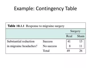
Gender (X)Smoke (Y) Male Female Total Yes 239 80 319 No 174 523 697Total 413 603 1,016Lambda = 0.4720,Chi Square = 226.3868
(1) Covariation and (2) time order [zero-order]X Y t1 t2
Respondents Under the Age of 40 (Z1)Gender (X)Smoke (Y) Male Female Total Yes 143 48 191 No 104 314 418Total 247 362 609Lambda = 0.4724,Chi Square = 135.8831
Respondents 40 Years of Age and Over (Z2)Gender (X)Smoke (Y) Male Female Total Yes 96 32 128 No 70 209 279Total 166 241 407Lambda = 0.4716,Chi Square = 90.5035
1. Replication (first-order partial) Z not-Z X Y X Y t1 t2 t1 t2
Respondents Under the Age of 40 (Z1)Gender (X)Smoke (Y) Male Female Total Yes 152 152 304 No 152 153 305Total 304 305 609Lambda = 0.0016,Chi Square = 0.0013
Respondents 40 Years of Age and Over (Z2)Gender (X)Smoke (Y) Male Female Total Yes 101 102 203 No 102 102 204Total 203 204 407Lambda = 0.0024,Chi Square = 0.0024
2. “Washed out” (first-order partial) [statistical independence of X and Y] Z not-Z X Y X Y t1 t2 t1 t2
Respondents Under the Age of 40 (Z1)Gender (X)Smoke (Y) Male Female Total Yes 164 140 304 No 156 149 305Total 320 289 609Lambda = 0.0281,Chi Square = 0.4786
Respondents 40 Years of Age and Over (Z2)Gender (X)Smoke (Y) Male Female Total Yes 173 31 204 No 30 173 203Total 203 204 407Lambda = 0.7003,Chi Square = 199.5759
3. Specification (first-order partial) Z not-Z X Y X Y t1 t2 t1 t2
Problems with the Elaboration Model·the greatest difficulty is running out of cases with multiple control variables with control variables having multiple categories with polytomous variables anywhere·thus, tends to be used with ONE control variable as a time; not a true evaluation of causality·difficulty of interpretation in complex tables·how “different” is “different” in concluding specification versus some form of explanation
Using SAS to Perform Multiple Contingency-Table Analysislibname old 'a:\';libname library 'a:\';options formchar='----|+|---+=|-/\<>*' ps=66 nodate nonumber;proc freq data=old.cities;table crimes*cityspnd / all;title1 'Multiple Contingency Table Analysis';title2;title3 'Zero-Order Table';run;proc sort data=old.cities out=temp;bycitysize;run;proc freq data=temp;table crimes*cityspnd / all;bycitysize;title1 'Multiple Contingency-Table Analysis';title2;title3 'First-Order Partial Tables';run;
Multiple Contingency-Table Analysis Zero-Order Table TABLE OF CRIMES BY CITYSPND CRIMES(CRIME RATE, DICHOTOMY) CITYSPND(CITY SPENDING, DICHOTOMY) Frequency| Percent | Row Pct | Col Pct |Less |More | Total ---------+--------+--------+ Lo_Crime | 24 | 11 | 35 | 38.10 | 17.46 | 55.56 | 68.57 | 31.43 | | 55.81 | 55.00 | ---------+--------+--------+ Hi_Crime | 19 | 9 | 28 | 30.16 | 14.29 | 44.44 | 67.86 | 32.14 | | 44.19 | 45.00 | ---------+--------+--------+ Total 43 20 63 68.25 31.75 100.00
Multiple Contingency-Table Analysis Zero-Order Table STATISTICS FOR TABLE OF CRIMES BY CITYSPND Statistic DF Value Prob ------------------------------------------------------Chi-Square 1 0.0040.952 Likelihood Ratio Chi-Square 1 0.004 0.952 Continuity Adj. Chi-Square 1 0.000 1.000 Mantel-Haenszel Chi-Square 1 0.004 0.952 Fisher's Exact Test (Left) 0.631 (Right) 0.582 (2-Tail) 1.000 Phi Coefficient 0.008 Contingency Coefficient 0.008 Cramer's V 0.008 Statistic Value ASE ------------------------------------------------------ Gamma 0.016 0.272 Kendall's Tau-b 0.008 0.126 Stuart's Tau-c 0.007 0.117 Somers' D C|R 0.007 0.118Somers' D R|C0.008 0.135 Pearson Correlation 0.008 0.126 Spearman Correlation 0.008 0.126 Lambda Asymmetric C|R 0.000 0.000 Lambda Asymmetric R|C 0.000 0.000 Lambda Symmetric 0.000 0.000 Uncertainty Coefficient C|R 0.000 0.002 Uncertainty Coefficient R|C 0.000 0.001 Uncertainty Coefficient Symmetric 0.000 0.001
Multiple Contingency-Table Analysis First-Order Partial Tables----------------------- SIZE OF CITY, DICHOTOMY=Small ------------------------ TABLE OF CRIMES BY CITYSPND CRIMES(CRIME RATE, DICHOTOMY) CITYSPND(CITY SPENDING, DICHOTOMY) Frequency| Percent | Row Pct | Col Pct |Less |More | Total ---------+--------+--------+ Lo_Crime | 19 | 9 | 28 | 42.22 | 20.00 | 62.22 | 67.86 | 32.14 | | 57.58 | 75.00 | ---------+--------+--------+ Hi_Crime | 14 | 3 | 17 | 31.11 | 6.67 | 37.78 | 82.35 | 17.65 | | 42.42 | 25.00 | ---------+--------+--------+ Total 33 12 45 73.33 26.67 100.00
Multiple Contingency-Table Analysis First-Order Partial Tables----------------------- SIZE OF CITY, DICHOTOMY=Small ------------------------ STATISTICS FOR TABLE OF CRIMES BY CITYSPND Statistic DF Value Prob ------------------------------------------------------Chi-Square 1 1.1370.286 Likelihood Ratio Chi-Square 1 1.184 0.277 Continuity Adj. Chi-Square 1 0.516 0.472 Mantel-Haenszel Chi-Square 1 1.111 0.292 Fisher's Exact Test (Left) 0.239 (Right) 0.924 (2-Tail) 0.488 Phi Coefficient -0.159 Contingency Coefficient 0.157 Cramer's V -0.159 Statistic Value ASE ------------------------------------------------------ Gamma -0.377 0.323 Kendall's Tau-b -0.159 0.139 Stuart's Tau-c -0.136 0.121 Somers' D C|R -0.145 0.128Somers' D R|C-0.174 0.152 Pearson Correlation -0.159 0.139 Spearman Correlation -0.159 0.139 Lambda Asymmetric C|R 0.000 0.000 Lambda Asymmetric R|C 0.000 0.000 Lambda Symmetric 0.000 0.000 Uncertainty Coefficient C|R 0.023 0.040 Uncertainty Coefficient R|C 0.020 0.035 Uncertainty Coefficient Symmetric 0.021 0.038
Multiple Contingency-Table Analysis First-Order Partial Tables----------------------- SIZE OF CITY, DICHOTOMY=Large ------------------------ TABLE OF CRIMES BY CITYSPND CRIMES(CRIME RATE, DICHOTOMY) CITYSPND(CITY SPENDING, DICHOTOMY) Frequency| Percent | Row Pct | Col Pct |Less |More | Total ---------+--------+--------+ Lo_Crime | 5 | 2 | 7 | 27.78 | 11.11 | 38.89 | 71.43 | 28.57 | | 50.00 | 25.00 | ---------+--------+--------+ Hi_Crime | 5 | 6 | 11 | 27.78 | 33.33 | 61.11 | 45.45 | 54.55 | | 50.00 | 75.00 | ---------+--------+--------+ Total 10 8 18 55.56 44.44 100.00
Multiple Contingency-Table Analysis First-Order Partial Tables----------------------- SIZE OF CITY, DICHOTOMY=Large ------------------------ STATISTICS FOR TABLE OF CRIMES BY CITYSPND Statistic DF Value Prob ------------------------------------------------------Chi-Square 1 1.1690.280 Likelihood Ratio Chi-Square 1 1.197 0.274 Continuity Adj. Chi-Square 1 0.354 0.552 Mantel-Haenszel Chi-Square 1 1.104 0.293 Fisher's Exact Test (Left) 0.943 (Right) 0.278 (2-Tail) 0.367 Phi Coefficient 0.255 Contingency Coefficient 0.247 Cramer's V 0.255 Statistic Value ASE ------------------------------------------------------ Gamma 0.500 0.387 Kendall's Tau-b 0.255 0.223 Stuart's Tau-c 0.247 0.218 Somers' D C|R 0.260 0.227Somers' D R|C0.250 0.220 Pearson Correlation 0.255 0.223 Spearman Correlation 0.255 0.223 Lambda Asymmetric C|R 0.125 0.388 Lambda Asymmetric R|C 0.000 0.452 Lambda Symmetric 0.067 0.363 Uncertainty Coefficient C|R 0.048 0.086 Uncertainty Coefficient R|C 0.050 0.089 Uncertainty Coefficient Symmetric 0.049 0.087
Causal Modeling with Discrete VariablesAttached are (selected) hypothetical output from three crosstabulations conducted using SAS. The first is the result of a (zero-order) crosstabulation between serious crimes per 1,000 population (CRIME) and per capita income (INCOME) for a random sample of 63 cities in the United States. The second and third results are for the crosstabulation of crime and per capita income with size of city, large and small respectively (CITYSIZE), held constant. In this exercise, CRIME is the dependent variable (Y), INCOME is the independent variable (X), and CITYSIZE is the control variable (Z). Assume the following time order among the three variables: CITYSIZE precedes INCOME which precedes CRIME. Set a = 0.05 and answer the following questions.1. Is the criterion of covariation between INCOME and CRIME satisfied by the zero-order crosstabulation? ________2. Is the relationship between INCOME and CRIME spurious based upon the results in the partial tables? ________3. How would you describe the relationship between the three variables, INCOME, CRIME, and CITYSIZE?
Results for Zero-Order Table TABLE OF INCOME (ROWS) BY CRIME (COLUMNS) TEST STATISTIC VALUE DF PROB PEARSON CHI‑SQUARE 5.818 1 .039 COEFFICIENT VALUE LAMBDA .3427 Results for First-Order Partial Table Large Cities ONLY TABLE OF INCOME (ROWS) BY CRIME (COLUMNS) FOR THE FOLLOWING VALUES: CITYSIZE = 1 (Large) TEST STATISTIC VALUE DF PROB PEARSON CHI‑SQUARE 4.967 1 .041 COEFFICIENT VALUE LAMBDA .2996 Results for First-Order Partial Table Small Cities ONLY TABLE OF INCOME (ROWS) BY CRIME (COLUMNS) FOR THE FOLLOWING VALUES: CITYSIZE = 0 (Small) TEST STATISTIC VALUE DF PROB PEARSON CHI‑SQUARE 4.833 1 .044 COEFFICIENT VALUE LAMBDA .2895
Causal Modeling with Discrete VariablesAttached are (selected) hypothetical output from three crosstabulations conducted using SAS. The first is the result of a (zero-order) crosstabulation between serious crimes per 1,000 population (CRIME) and per capita income (INCOME) for a random sample of 63 cities in the United States. The second and third results are for the crosstabulation of crime and per capita income with size of city, large and small respectively (CITYSIZE), held constant. In this exercise, CRIME is the dependent variable (Y), INCOME is the independent variable (X), and CITYSIZE is the control variable (Z). Assume the following time order among the three variables: CITYSIZE precedes INCOME which precedes CRIME. Set a = 0.05 and answer the following questions.1. Is the criterion of covariation between INCOME and CRIME satisfied by the zero-order crosstabulation? Yes2. Is the relationship between INCOME and CRIME spurious based upon the results in the partial tables? Yes3. How would you describe the relationship between the three variables, INCOME, CRIME, and CITYSIZE? CITYSIZE causes both INCOME and CRIME


