Predator-Prey Dynamics for Rabbits, Trees, & Romance
330 likes | 476 Vues
Predator-Prey Dynamics for Rabbits, Trees, & Romance. J. C. Sprott Department of Physics University of Wisconsin - Madison Presented at the Swiss Federal Research Institute (WSL) in Birmendsdorf, Switzerland on April 29, 2002. Collaborators. Janine Bolliger

Predator-Prey Dynamics for Rabbits, Trees, & Romance
E N D
Presentation Transcript
Predator-Prey Dynamics for Rabbits, Trees, & Romance J. C. Sprott Department of Physics University of Wisconsin - Madison Presented at the Swiss Federal Research Institute (WSL) in Birmendsdorf, Switzerland on April 29, 2002
Collaborators • Janine Bolliger • Swiss Federal Research Institute • Warren Porter • University of Wisconsin • George Rowlands • University of Warwick (UK)
Rabbit Dynamics • Let R = # of rabbits • dR/dt = bR - dR = rR r = b - d Birth rate Death rate • r > 0 growth • r = 0 equilibrium • r < 0 extinction
Exponential Growth • dR/dt = rR • Solution: R = R0ert R r > 0 r = 0 # rabbits r < 0 t time
Logistic Differential Equation • dR/dt = rR(1 - R) 1 R r > 0 # rabbits 0 t time
Effect of Predators • Let F = # of foxes • dR/dt = rR(1 - R - aF) Intraspecies competition Interspecies competition But… The foxes have their own dynamics...
Lotka-Volterra Equations • R = rabbits, F = foxes • dR/dt = r1R(1 - R - a1F) • dF/dt = r2F(1 - F - a2R) r and a can be + or -
Types of Interactions dR/dt = r1R(1 - R - a1F) dF/dt = r2F(1 - F - a2R) + a2r2 Prey- Predator Competition - + a1r1 Predator- Prey Cooperation -
Equilibrium Solutions • dR/dt = r1R(1 - R - a1F) = 0 • dF/dt = r2F(1 - F - a2R) = 0 Equilibria: • R = 0, F = 0 • R = 0, F = 1 • R = 1, F = 0 • R = (1 - a1) / (1 - a1a2), F = (1 - a2) / (1 - a1a2) F R
Stable Focus(Predator-Prey) r1(1 - a1) < -r2(1 - a2) r1 = 1 r2 = -1 a1 = 2 a2 = 1.9 r1 = 1 r2 = -1 a1 = 2 a2 = 2.1 F F R R
Stable Saddle-Node(Competition) a1 < 1, a2 < 1 r1 = 1 r2 = 1 a1 = 1.1 a2 = 1.1 r1 = 1 r2 = 1 a1 = .9 a2 = .9 Node Saddle point F F Principle of Competitive Exclusion R R
Coexistence • With N species, there are 2N equilibria, only one of which represents coexistence. • Coexistence is unlikely unless the species compete only weakly with one another. • Diversity in nature may result from having so many species from which to choose. • There may be coexisting “niches” into which organisms evolve. • Species may segregate spatially.
Reaction-Diffusion Model • Let Si(x,y) be density of the ith species (rabbits, trees, seeds, …) • dSi/ dt = riSi(1 - Si - ΣaijSj) + Di2Si ji reaction diffusion where 2Si = Sx-1,y + Sx,y-1 + Sx+1,y + Sx,y+1 - 4Sx,y 2-D grid:
Alternate Spatial Lotka-Volterra Equations • Let Si(x,y) be density of the ith species (rabbits, trees, seeds, …) • dSi/ dt = riSi(1 - Si - ΣaijSj) ji where S = Sx-1,y + Sx,y-1 + Sx+1,y + Sx,y+1 + aSx,y 2-D grid:
Parameters of the Model Growth rates Interaction matrix 1 r2 r3 r4 r5 r6 1 a12a13a14a15a16 a21 1 a23a24a25a26 a31a32 1a34a35a36 a41a42a43 1a45a46 a51a52a53a54 1a56 a61a62a63a64a65 1
Features of the Model • Purely deterministic (no randomness) • Purely endogenous (no external effects) • Purely homogeneous (every cell is equivalent) • Purely egalitarian (all species obey same equation) • Continuous time
Fluctuations in Cluster Probability Cluster probability Time
Power Spectrumof Cluster Probability Power Frequency
Fluctuations in Total Biomass Time Derivative of biomass Time
Power Spectrumof Total Biomass Power Frequency
Sensitivity to Initial Conditions Error in Biomass Time
Results • Most species die out • Co-existence is possible • Densities can fluctuate chaotically • Complex spatial patterns spontaneously arise One implies the other
Romance(Romeo and Juliet) • Let R = Romeo’s love for Juliet • Let J = Juliet’s love for Romeo • Assume R and J obey Lotka-Volterra Equations • Ignore spatial effects
Romantic Styles dR/dt = rR(1 - R - aJ) + a Cautious lover Narcissistic nerd - + r Eager beaver Hermit -
Pairings - Stable Mutual Love Cautious Lover Eager Beaver Narcissistic Nerd Hermit Narcissistic Nerd 46% 67% 5% 0% Eager Beaver 67% 39% 0% 0% Cautious Lover 5% 0% 0% 0% Hermit 0% 0% 0% 0%
Love Triangles • There are 4-6 variables • Stable co-existing love is rare • Chaotic solutions are possible • But…none were found in LV model • Other models do show chaos
Summary • Nature is complex • Simple models may suffice but
http://sprott.physics.wisc.edu/ lectures/predprey/ (This talk) sprott@juno.physics.wisc.edu References