Download
1 / 50
500 likes | 628 Vues
Theoretical Modeling for the STEREO Mission. Markus Aschwanden et al. Lockheed Martin Solar & Astrophysics Laboratory. Solar-B/STEREO Workshop, Turtle Bay Resort, Oahu, Hawaii – Nov 15-18, 2005. Ref.: Aschwanden et al. (2005), Space Science Rev., (subm.)

E N D
TheoreticalModeling for the STEREO Mission Markus Aschwanden et al. Lockheed Martin Solar & Astrophysics Laboratory Solar-B/STEREO Workshop, Turtle Bay Resort, Oahu, Hawaii – Nov 15-18, 2005 Ref.: Aschwanden et al. (2005), Space Science Rev., (subm.) http://www.lmsal.com/~aschwand/publications/eprints/2005_stereobook.pdf
et al.: GSFC: L.F.Burlaga, M.L.Kaiser, C.K.Ng, D.V.Reames, M.J. Reiner Univ.Michigan: T.I.Gombosi, N.Lugaz, W.IV.Ward Manchester, II.Roussev, T..H.Zurbuchen Univ.New Hampshire: C.J.Farrugia, A.Galvin, M.A.Lee SAIC: J.A.Linker, Z.Mikic, P.Riley Rice Univ: D.Alexander, A.W.Sandman NRL: J.W.Cook, R.A.Howard NOAA/SEC: D.Odstrcil, V.Pizzo JPL: P.C.Liewer, E.DeJong UCB: J. Luhmann MPIS: B.Inhester, R.W.Schwenn, S.Solanki, V.M.Vasyliunas, T.Wiegelmann Univ.Bern: L.Blush, P.Bochsler Univ.Sydney: I.H.Cairns, P.A.Robinson Univ.Goettingen: V.Bothmer KFIK RMKI, Budapest, Hungary: K.Kecskemety Univ.Arizona: J.Kota CNRS: A. Llebaria CNRS, LESIA: Maksimovic MPES: M.Scholer Univ. Kiel: R.Wimmer-Schweingruber
1. Modeling the Solar Corona Schrijver, Sandman, Aschwanden, & DeRosa (2004)
A full-scale 3D model of the solar corona: • (Schrijver et al. 2004) • 3D magnetic field model (using Potential source • surface model) computed from synoptic (full-Sun) • photospheric magnetogram10^5 loop structures • -Coronal heating function • E_H(x,y,z=0)~B(x,y)^a*L(x,y)^b a~1, b~-1 • -Hydrostatic loop solutions • E_H(s)-E_rad(s)-E_cond(s)=0 • yield density n_e(s) and T_e(s) profiles • -Line-of-sight integration yields DEM for every • image pixel • dEM(T,x,y)/ds = Int[ n_e^2(x,y,z,T[x,y,z])] dz • -Free parameters can be varied until synthetic image • matches observed ones in each temperature filter • -STEREO will provide double constraint with two • independent line-of-sights.
Hydrostatic/hydrodynamic modeling of coronal loops requires careful disentangling of neighbored loops, background modeling, multi-component modeling, and multi-filter temperature modeling. Accurate modeling requires the identification of elementary loops.
Inversion of coronal density with coarse • Resolution (~15 heliographic deg): • White light inversion (Thomson scattering) • Van de Hulst (1950) • Lamy et al. (1997) • Llebaria et al. (1999) • -Soft X-ray tomography • Hurlburt et al. (1994) • Davila (1994) • Zidowitz (1997) • Numerical MHD simulations (~1” pixels): • Gudiksen & Nordlund (2002, 2005) • Mok et al. (2005)
Stereoscopic reconstruction of coronal loops, 3D-geometry: -Loughhead, Wang & Blows (1983) -Berton & Sakurai (1985) Tie-point method: -Liewer et al. (2000) -Hall et al. (2004) Solar-rotation stereoscopy: -Koutchmy & Molodensky (1992) -Vedenov et al. (2000) Dynamic stereoscopy: -Aschwanden et al. (1999, 2000) Magnetic field-aided reconstruction: -Gary & Alexander (1999) -Wiegelmann & Neukirch (2002) -Wiegelmann & Inhester (2003) -Wiegelmann et al. (2005)
3D-reconstruction of coronal loop structures to test theoretical models of magnetic field extrapolations.
Fingerprinting (automated detection) of curvi-linear structures • Lee, Newman & Gary • improve detection of • coronal loops with • “Oriented connectivity • Method” (OCM): • median filtering • contrast enhancement • unsharp mask • detection threshold • directional connectivity Lee, Newman, & Gary (2004), 17th Internat. Conf. On Pattern Recognition, Cambridge UK, 23-26 Aug 2004
Elementary vs. Composite loops: • Each loop strand represents an “isolated mini-atmosphere” • and has its own hydrodynamic structure T(s), n_e(s), • which needs to be extracted by subtracting it from the • background coronal structures. • SECCHI/EUVI (1.6” pixels) will be able to resolve some individual loops, substantially better than CDS (4” pixels), but somewhat less than TRACE (0.5” pixels).
Loops Widths Loop/Backgr. Instrument Ref. • 1 ~12 Mm ? CDS Schmelz et al. (2001) • ? 170%150% EIT Schmelz et al. (2003) • 7.10.8 Mm 30%20% EIT Aschwanden et al. (1999) • 1 ~5.8 Mm 76%34% TRACE/CDS DelZanna & Mason (2003) • 3.71.5 Mm ? TRACE Aschwanden et al. (2000) • (no highpass filter) • 1.40.2 Mm 8%3% TRACE Aschwanden & Nightingale • 2005 (with highpass filter)
Model: Forward- Fitting to 3 filters varying T
Elementary Loop Strands The latest TRACE study has shown the existence of elementary loop strands with isothermal cross-sections, at FWHM widths of <2000 km. TRACE has a pixel size of 0.5” and a point-spread function of 1.25” (900 km) and is able to resolve them, while EUVI (1.6” pixels, PSF~3.2”=2300 km) will marginally resolve the largest ones. Triple-filter analysis (171, 195, 284) is a necessity to identify these elementary loop strands. Aschwanden & Nightingale (2005), ApJ 633 (Nov issue)
The advantage of STEREO is that a loop can be mapped from two different directions, which allows for two independent background subtractions. This provides an important consistency test of the loop identity and the accuracy of the background flux subtraction. A B F b F a x x Consistency check: Is F_a = F_b ?
PFSS-models (Potential Field Source Surface) are used to compute full-Sun 3D magnetic field (current-free xB=0) Open fields occur not only in coronal holes, but also in active regions escape paths of energized particles into interplanetary space Schrijver & DeRosa (2003) find that ~20%-50% (solar min/max) of interplanetary field lines map back to active regions. Schrijver & DeRosa (2003)
SAIC Magnetohydrodymanics Around a Sphere (MAS)-code models magnetic field B(x,y,z) solar wind speeds v(x,y,z) in range of 1-30 solar radii from synoptic magnetogram Model computes stationary solution of resistive MHD Equations n_e, T_e, p, B MAS model simulates coronal streamers (Linker, vanHoven, Schnack1990) Line-of-sight integration yields white-light images for SECCHI/ COR and HI
SAIC/MAS-IP code combines corona (1-30 solar radii) and Inner heliosphere (30 Rs -5 AU) Model reproduces heliospheric current sheet, speeds of fast & slow solar wind, and interplanetary magnetic field NOAA/ENLIL code (Odstrcil et Al. 2002) is time-dependent 3D MHD code (flux-corrected transport algorithm): inner boundary is sonic point (21.5-30 Rs from WSA code, outer boundary is 1-10 AU.
SMEI heliospheric tomography model uses interplanetary scintillation (IPS) data for reconstruction of solar wind (Jackson & Hick 2002) Exospheric solar wind model computes proton and electron Densities in coronal holes In range of 2-30 Rs (Lamy et al. 2003) Univ.Michigan solar wind code models solar wind with a sum of potential and nonpotential Magnetic field components (Roussev et al. 2003)
3. Modeling of Erupting Filaments Roussev et al. (2003)
Pre-eruption conditions of filaments Envold (2001) Aulanier & Schmieder (2002) • Geometry and multi-threat structure of filaments • (helicity, chirality, handedness conservation, fluxropes) • Spatio-temporal evolution and hydrodynamic balance • Stability conditions for quiescent filaments • Hydrodynamic instability and magnetic instability • of erupting filaments leading to flares and CMEs
Measuring the twist of magnetic field lines Aschwanden (2004) • Measuring the number of turns in twisted loops • Testing the kink-instability criterion for stable/erupting loops • Monitoring the evolution of magnetic relaxation (untwisting) • between preflare and postflare loops
Measuring the twist of magnetic field lines Aschwanden (2004) • Measuring number of turns in (twisted) sigmoids • before and after eruption • -Test of kink-instability criterion as trigger of flares/CMEs
Measuring the twist of erupting fluxropes Gary & Moore (2004) • Measuring number of turns in erupting fluxropes • -Test of kink-instability criterion as trigger of flares/CMEs
Triggers for of filaments or Magnetic flux ropes: -draining of prominence material bouancy force (Gibson & Low 1998) (Manchester et al. 2004) -current increase and loss of equilibrium (Titov & Demoulin 1999) (Roussev, Sokolov, & Forbes) (Roussev et al. 2003) -kink instability unstable if twist > 3.5 (Toeroek & Kliem 2003, Toeroek, KIiem, & Titov 2003)
MHD simulations of coronal dimming: -evacuation of plasma beneath CME, fast-mode MHD wave (Wang 2000; Chen et al. 2002; Wu et al. 2001)
5. Modeling of Coronal Mass Ejections (CMEs) pB MAS/ENLIL code streamer, eruption and evolution of CME (Mikic & Linker 1994; Lionello et al. 1998; Mikic et al. 1999) Linker et al. 1999)
BATS`R’US-code (ideal MHD code) Simulates launch of CME by loss of equilibrium of fluxrope (Roussev et al. 2004; Lugaz, Manchester & Gombosi 2005)
ENLIL+MAS code: simulates propagation of CME in solar wind, produces accurate shock strenghts, arrival of shocks at 1 AU (Odstrcil et al. 1996, 2002 2004, 2005; Odstrcil & Pizzo 1999)
3D Reconstruction from 2 STEREO images (either from EUVI or white-light coronagraphs) z CME y 3D Reconstruction Volume x (0,0,0) x x-y plane coplanar with STEREO spacecraft A and B Sun
Slices with independent 2D reconstructions : - Adjacent solutions can be used as additional constraints
2D Slices of reconstruction from 2 views STEREO-B STEREO-A
Is 2D reconstruction from two projections unique ? Coordinate rotation (x,y) (u,v) : u y v x (STEREO-B) (STEREO-A) INVERSION
6. Modeling of Interplanetary Shocks Odstrcil & Pizzo (1999)
Fast CMEs have speeds of v>2000 km/s formation of fast-mode shock Numerical MHD simulations: - Mikic & Linker (1994) - Odstrcil & Pizzo (1999) - Odstrcil, Pizzo, & Arge (2005) Predicted arrival time at 1 AU depends critically on models of background solar wind which controls shock propagation speed - Odstrcil, Pizzo & Arge (2005) CME cannibalism (faster overtakes slower one) compound streams, interactions with CIR (corotating interaction regions) control shock-accelerated particles (SEPs) Odstrcil & Pizzo (1999)
7. Modeling of Interplanetary Particle Beams and Radio Emission
Interplanetary radio emission • (see also talk by J-L. Bougeret) • electron beams type III • shock waves type II • IP space is collisionless • -propagation of suprathermal • electron and ion beams • velocity dispersion • bump-in-tail instability • Langmuir wave growth at • fundamental + harmonic • plasma frequency (f_p~n_e^1/2) • stochastic growth theory • Robinson & Cairns (1998) Pocquerusse et al. (1996)
Type II bursts do not outline entire shock front, but occur only where shock wave intersects preexisting structures Reiner & Kaiser (1999) Interplanetary type II bursts were All found to be associated with fast CMEs, with shock transit Speeds v>500 km/s Cane, Sheeley, & Howard (1987) Semi-quantitative theory of type II bursts includes magnetic mirror reflection and acceleration of upstream electrons incident on shock (Knock & Cairns 2005)
In-situ particle + remote sensing (IMPACT + SWAVES) (courtesy of Mike Reiner)
8. Modeling of Solar Energetic Particles (SEPs) (see also talks by J.Luhmann and R.Mewaldt)
-Two-point in-situ measurements acceleration of flare particles (A) versus acceleration in CME-driven shocks (B) -Efficiency of quasi-parallel vs. quasi-perpendicular shock acc. -Time-of-flight measurements at two spacecraft and Earth localization of acceleration sources (flare, CME, CIR, CME front, preceding shock, CME flank, etc.) -Quadrature observations shock profile (A) and in-situ (B)
Theoretical modeling of SEPs: Diffusive shock acceleration, proton-excited Alfvenic waves upstream of shock, escape of particles upstream of the shock by magnetic focusing (Marti Lee, 2005) SEP propagation over several AU, fast acceleration by coronal shock, co-evolution of Alfven waves in inhomogeneous IP, focusing, convection, adiabatic deceleration, scattering by Alfven waves SEP fluxes and spectra Modeling for STEREO/IMPACT Tylka, Reames, & Ng (1999) (Chee Ng & Don Reames)
9. Modeling of Geo-effective events and Space Weather -Arrival time of shocks at Earth will be improved by 3D triangulation of CME propagation with two spacecraft (STEREO 3D v-vector and r-vector reconstruction vs. LASCO CME speed (lower limit) projected in plane of sky -End-to-end models attempted including MHD of lower corona, heliosphere, and magnetosphere + SEP accel. & propagation - CCMC (Community Coordinated Modelin Center, GSFC) - CISM (Center for Integrated Space Weather Modeling, UCB) - CSEM (Center for Space Environment Modeling, UMich) - Solar/Muri (Solar Multidisciplinary Univ. Research Initiative)
CONCLUSIONS • Theory and modeling efforts for the STEREO mission is • designed for data data analysis of both remote-sensing • (SECCHI, SWAVES) and in-situ instruments (IMPACT, • PLASTIC). • -Modeling includes background plasma in corona, • heliosphere, and solar wind, but concentrates on • dynamic phenomena associated with initiation of CMEs • in lower corona (filament dynamics, shearing, kinking, • loss-of-equilibrium, filament eruption, magnetic • reconnection in coronal flare sites), and propagation • and evolution of CMEs in interplanetary space • (interplanetary shocks, IP particle beams, SEP • acceleration and propagation, geoeffective events, • space weather), attempting end-to-end models from • corona, trhough heliosphere, to magnetosphere).