Download
1 / 59
610 likes | 806 Vues
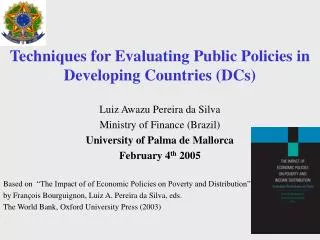
Techniques for Evaluating Public Policies in Developing Countries (DCs). Luiz Awazu Pereira da Silva Ministry of Finance (Brazil) University of Palma de Mallorca February 4 th 2005 Based on “The Impact of of Economic Policies on Poverty and Distribution”

E N D
Techniques for Evaluating Public Policies in Developing Countries (DCs) Luiz Awazu Pereira da Silva Ministry of Finance (Brazil) University of Palma de Mallorca February 4th 2005 Based on “The Impact of of Economic Policies on Poverty and Distribution” by François Bourguignon, Luiz A. Pereira da Silva, eds. The World Bank, Oxford University Press (2003)
Outline of this Presentation • Policy Challenges for DCs: the evaluation of public expenditures and economic policies from aggregate macro to micro “distribution/poverty” • Framework for evaluating public policies • Part 1 : Microeconomic evaluation techniques • Part 2 : Macro evaluation techniques (micro-macro linkages) • Future directions for more complex techniques • Practical difficulties for DCs (institutional set-up)
Evaluation techniques in DCs have evolved together with: • Development Economics, e.g., goals and theory • Data Availability and Econometric Techniques, e.g., HHS, Firm data • Modeling techniques, e.g., CBA, CGEs • Challenges of Globalization , e.g., political economy in DCs • Policy Challenges for DCs now: linking the evaluation of public expenditures, economic policies to “distribution/poverty”
Policy Challenges: 1950-1970s “old” vision of Evaluation of Public Policies • Maximize Aggregate Growth and Minimize Risks of BoP crisis, under old BW international financial arquitecture (fixed ERs, K controls, etc.) and import-substituting development strategies • Evaluation = from aggregate growth models level of external savings needed for target growth, Kflows (public), find the best set of projects doing project analysis in partial equilibrium (CBA) using if need be shadow-pricing • Most DCs with institutional structure for evaluation with strong Min. Planning and Project Analysis Unit (World Bank, IMF) and MoF in control of ER, BoP
Policy Results (1970s-1980s) of “old” vision of Evaluation of Public Policies • Some successes but also booms and busts Policy instability, structural adjustments, external vulnerability • Fiscal and/or BoP crises high or hyper inflation, devaluations • Poverty and distributional challenges Political instability • Shift in institutional balance: MoFs vs. Planning • Obsolescence of most project analysis units and of CBA in planning & evaluation methods
Policy Challenges 1990s-2000s (1): the most common economic policies and structural reforms in DCs change in scope for Evaluation of Public Policies • Macro-economic policies, ST Fiscal monetary policy stance, exchange rate regime, public debt management strategy, etc. • Public Expenditure and Revenue, Micro-social-policies, ST - MT Tax policy reform, composition of public expenditure, design of social programs (CCTs) civil service reform, pension reform, decentralization • Structural Reforms, LT Trade liberalization, liberalization of specific markets, financial sector reforms, improving the investment climate, land reform, privatization etc.
Within point 2., in particular, most common policy challenge for DCs is Evaluation of Public Expenditure • Adequate Aggregate Level Is Deficit, Public debt Sustainable? • Definition of PS, Hidden Contingent Liabilities? • Methodology (mechanical ratios or stochastic)? • Adequate dynamics, counter-cyclicality of public spending? • Macro policy fiscal stance and “credibility” • Programs to off-set effect of volatility, financial crises • Is there crowding-out or crowding in private/public? • Complementarity of PE,Externalities w/ private sector? • Market failures? Lobbies? • Are allocations adequate? • Inter-sectoral allocation, Capacity-building • Input mix (Capital/Recurrent; Wage/Non-Wage) • What are Poverty and Distributional Impact of PE? • Cost-Efficiency of social programs • Outcome indicators, Evaluation methods
Illustration of Typical Set of Challenges for DCs: Example of Brazil • High PS Debt and unsustainable Tax Burden Need to Generate Primary Fiscal Surpluses • High and persistent inequality, poverty and Budget rigidity Need to Improve Targeting of Social Policies
Tax/GDP Public Debt/GDP Gini
Evaluation of Policies in DCs with these new policy challenges: broader range of micro programs to macro policies • Scope and objective, challenges increase: evaluate the economic feasibility of public programs and policies and their overall ‘development” impact. • Aggregate and first principle analysis insufficient: heterogeneity of individuals and households, microeconomic behavior do not add up into aggregate nor “average”, specificities of economic structures and local political economy, transmission of shocks and policies • Policy objectives and social demand increasingly focusing on distributional effects and poverty reduction, essentially micro concepts (e.g., Post-WC IFIs, new types of Governments, etc.) • Micro data bases (household surveys HHS) increasingly available as the natural analytical environment for distributional and poverty analysis • Hence the natural idea to link the effect of economic policies to the corresponding changes in the income and/or expenditure of individuals, households, social groups and the poor in particular • Impact evaluation allows to think about “scaling-up” and pro-poor, redistributive development strategies
Important dimensions in the evaluation of Public Policies in DCs with these new policy challenges • Counterfactual is needed (the world with and without the program or policy being evaluated, sometimes difficult) • Ex-ante or ex-post (ex-ante evaluates the design of non-existing programs and policies, ex-post focus on outcomes) • Partial or General Equilibrium (taking or not into account the effect of programs and policies on price systems and economic equilibria) • Behavioral or “Arithmetic” (based or not into some representation of economic behavior of agents “reacting” to the program or policy )
Framework for Evaluation Define impact for individual i as the difference in income yi with and without the program, denominated Dyi : yi : real income wi : wage rate Li : labor supply Ei : self-employment, non-wage income Ri : net transfer income Ai : socio-economic characteristics Ci : consumption characteristics household-specific P price index p : general price index
Program or policy will shock one or more components that explain the individual income yi • A households character. • R transfers • p prices • w wage • L employt. Household Survey (HHS), i individual households Evaluation of Program and/or Economic Policy • Compare the distribution of y|P=1 with the distribution of y|P=0. • Calculate changes in inequality or poverty across the two distributions • Different tools/methods differ in how they construct the counterfactual distribution and the data that are needed • Rank results according to some agreed upon rule and/or objective
An illustration of one criteria for evaluation An incidence effect curve (say on income/ expenditure changes) showing the percent change in per capita income of a macroeconomic policy (here, Indonesia financial crisis, changes in pc income by percentiles of the distribution) poor wealthy
Part 1 “Microeconomic techniques” 1. Average Incidence Analysis • Tax Incidence Analysis (Sahn & Younger) • Public Expenditure Incidence Analysis (Demery) 2. Marginal Incidence Analysis • Behavioral response to changes (Van de Walle) • Poverty mapping (Lanjouw) 3. Impact Evaluation (randomization, matching, double-dif) a) Ex-post (Ravallion) b) Ex-ante (Bourguignon & Ferreira) 4. Data and Measurement (not covered here) a) Multi-topic Household Surveys(Scott) b) Qualitative surveys (Rao & Woolcock) c) Performance in Service Delivery (Dehn, Reinikka & Svensson)
Average Incidence Analysis (Sahn & Younger; Demery) • Suitable for taxes or public expenditures. • Aims to answer: “Who pays for / receives how much?” • Counterfactual is simply • So that • This is equivalent to assuming: • No behavioral response (perfectly inelastic demand for goods, perfectly inelastic supply of factors. • Fine for marginal changes. • But only a first order approximation to large taxes and/or transfers. • No general equilibrium effects.
Average Incidence Analysis (Sahn & Younger; Demery) • A practical example from education expenditures: the incidence of public spending in schooling category i which accrues to group j depends on: • groups j’s relative enrolment rates across schooling types i. • Relative spending across categories i. Once again: purely arithmetic. No behavioral response, no gen. eq. effects.
Marginal Incidence Analysis(van de Walle) • Suitable for taxes or public expenditures. • Aims to answer: “How has the distribution of tax burden / program benefits changed in the recent past?” • Assumptions are less demanding than for average incidence analysis • Requires either panel or repeated cross-section data. • Although some have suggested using spatial variation in programs / taxes to proxy for temporal variation (Lanjouw & Ravallion)
Poverty (and Expenditure) Maps (Lanjouw) Reliable poverty maps = combining sample survey data with census data to yield predicted poverty rates for all households covered by the census. 1) Estimating Models of Consumption A model of consumption or standard of living using household survey data is estimated using the variables which are available both in the census and in the survey. 2) Predicting Poverty. The parameter estimates from the regressions (using the full household sample) are used to predict consumption or standard of living in the census data. For each household in the census, the parameter estimates from the applicable regression (conditional on geographical location) are combined with the household's characteristics in order to obtain an imputed value for per capita consumption expenditure. 3) Comparing with the map of public expenditure spending. The poverty map that is obtained can then be “super-imposed” on the map for any public spending
Ex-Post Evaluation of public programs (Ravallion ) Randomization: Only a random sample is allowed to participate to the program. “Randomized out” group is the counterfactual. • Experiments may be either designed or natural: Progresa vs. Bolsa Alimentacao • Delayed participation of part of the population may be used to reach the same objective. • But beware of anticipation bias… • Randomization ensures that treatment and control groups are “alike” along all dimensions relevant for program selection, observable and unobservable. • Takes into account all partial and general equilibrium effects of program, as well as all behavioral responses. Ideal for measuring. Not so great at “explaining”.
Ex-Post Evaluation of public programs (Ravallion ) Matching: When no randomization is available, must construct a comparison group. Objective is to approximate a control: match participants to non-participants from a larger survey, on the basis of similarities in observed characteristics. • The most common method is to match people on the basis of their ex-ante probability to participate to the program, these probabilities depending on their characteristics as well as those of the communities they live in (Propensity-score matching): • Draws on seminal work by Rosenbaum and Rubin (1983)
Ex-Post Evaluation of public programs (Ravallion ) • Key problem with non-experimental data is that if any variables which affect selection into the program are not observed, they can not be included in X, and the approximation to the ideal counterfactual fails. • If two waves of data are available in time (I.e. with a baseline survey and a follow-up survey), then at least the time-invariant unobserved variables may be netted out through double differencing:
Ex-Ante Evaluation of public programs(Bourguignon & Ferreira) • Aims to simulate programs or program reforms which are not yet in existence. Complement to ex-post approach. • In this approach, the treatment –rather than the control – is the counterfactual. • The counterfactual incomes may be generated through: • Arithmetic micro-simulations (based on program rules) • Behavioral micro-simulations (based on a model)
Ex-Ante Evaluation of public programs(Bourguignon & Ferreira)
Public Expenditure Tracking Surveys Dehn, Reinnika and Svensson [2001] The need for special Public Expenditure Tracking Survey (PETS) comes primarily from the increasing evidence that budget allocations to social services (the basis for traditional “benefice incidence analysis”) are not consistent with the casual observation of what is really happening in the ground. • More evidence of government failures (corruption, leakages). • Little known about transformation of budgets into services (the public sector production function) • Household surveys show that quality of service important determinant of demand PETS gathers information on “flow of funds” within the public sector from: • Participatory poverty assessments • Service delivery surveys of households • Public officials surveys
Example : Education sector in Uganda 1996 • Data from 250 schools and administrative units • Only 13 percent of intended capitation grant actually reached schools (1991-95). • Mass information campaign by Ministry of Finance (the press, posters) • Follow-up surveys (PETS, provider surveys, integrity surveys, etc.) • High leakage has also been found in other countries (Tanzania, Ghana, Zambia, Peru)
Part 2 “Macroeconomic techniques”, from robust to more speculative…. 1. Standard RHG approaches to macro-micro linkage: • "Micro-accounting"/RHG approach based on aggregate macro predictions (PovStat-SimSip-PAMS) • The disaggregated SAM-CGE/RHG approach (Adelman-Robinson, Bourguignon and al. in the "Maquette“, Loefgren, Robinson or Agenor and al. with IMMPA.) 2. Top-down "micro-simulation" approaches (micro-macro linkages) • "Micro-accounting modules" linked to disaggregated macromodels(Chen-Ravallion, McCulloch-Winters) • "Micro-simulation modules" linked to disaggregated macro models (Bourguignon-Robilliard-Robinson, Ferreira-Leite-Pereira-Picchetti, Cogneau-Robilliard-van der Mensbrugghe) 3.Other issues for research and applications: a) Fully integrated models(Townsend, Heckman, Browning-Hansen-Heckman) b) Accounting for general equilibrium effects of public expenditure programs c) Dynamic modeling and the proper treatment of growth
Evaluation of macro economic policies.Macro to micro linkages Macro framework, general/partial equilibrium • A households character. • p prices • w wage • L employt. • R transfers Instead of « exogenous and independent » shocks like in Part 1, in Part 2 use « endogenous and dependent» shocks to 'microsimulate' the effect of policies on all individuals in the micro data sets, and the poor some consistency constraints will be « binding » (e.g., budget envelope for social programs, real GDP growth, etc.) LAVs =Linkage Aggregate Variables Household Survey (HHS), i individual households
Evaluation of macro economic policies. General approaches and problems • Before/after : evaluation based on the observation of changes in standards of living Dy inputed to some policy change affecting « jointly » (DL, DR, Dw, Dp, etc.) Problems Before/after evaluation techniques include other changes (DX)than policy (DL, DR,..) being evaluated difficulty to evaluate alternative policies by attributing changes to the effects of policy • Counterfactuals: Ideally possible to smulatechanges in standard of living due to alternative macroeconomic policies, e.g., (DE, Dr) during a BoP crisis Problems Program design/implementation in crisis time - credibility? • Top-to-Bottom approach: Linking macro to micro data using Linkage Aggregate Variables (LAVs) to simulate macro-to-micro effects consistently Problems Weakest link (macro? micro?), garbage in, garbage out and…
Evaluation of macro economic policies. General approaches and problems 1995 Nobel Laureate in Economics Robert E. Lucas Jr.
Standard RHG approaches to a macro-micro linkagea) "Micro-accounting"/RHG and aggregate macro predictions i. An elementary procedure Growth rate of output in sector k : gk Growth rate of employment in sector k : nk Effect on distribution (using a micro data base) given by: Multiply income of all hhs in sector k (or RHG) by: Reweigh all hhs in sector k (or RHG) by: Evaluate new distribution, all poverty and inequality measures ii. More elaborated models Change arbitrarily distribution within sector k Change distribution endogeneously by distinguishing labor/non-labor income, so that gk is not uniform anymore (PAMS, Pereira da Silva and alii) iii. Main problems = very much heterogeneity still missing + likely strong selection behind nk
Standard RHG approaches to a macro-micro linkageb) The SAM-CGE/RHG approach i. Basic idea Aggregation properties allow separating the household population into groups. Only the aggregate behavior of these groups matters for the (general) equilibrium of the economy. Overall distribution of income or earnings studied under the assumption that the distribution of 'relative' income within Representative Household Groups is constant – as given in a household survey - and also that their demographic weight is given. These approaches thus essentially focus on changes in the distribution between RHGs. ii. Working of standard (CGE) models (e.g., Robinson) Full integration of RHGs' behavior within the model: interaction of heterogeneous behavior in labor supply, consumption, savings, portfolio choice in the household sector with the production side and public policies through good and factor markets
Standard RHG approaches to a macro-micro linkage b) The SAM-CGE/RHG approach iii. Recent and current extensions Introduction of the monetary and financial sectors (IMMPA, Agenor and alii, Lewis & Robinson): Limited by current theoretical knowledge of the working of financial markets. Introducing imperfect competition indifferent ways : Economies of scale, economies of scope, oligopolistic behavior, bargaining on the labor market, … Dynamics represented through a sequence of temporary equilibria linked by asset accumulation and demographics
Standard RHG approaches to the macro-micro linkageb) The SAM-CGE/RHG approach iii. Limitations Miss 'true' intertemporal behavior and important sources of growth ( public expenditures in particular) Constant “within RHG” distribution limitative in a dynamic framework All improvements over simple static Walrasian case make all the more acute the issue of empirically 'calibrating' the model and the confidence one may have on predictions The 'black box' risk iv. Final Remarks These techniques are 'simple', yet they are not widely used They capture only the 'between' (RHG) dimension of distributional changes, which empirically proves limitative They are ill adapted to the distributional aspects of growth
2. Top-down "micro-simulation" approach within a macro-micro linkageapproach Macro model Linkage AggregatedVariables (prices, wages, employment levels) Household income micro-simulation model
2. Top-down "micro-simulation" approach within a macro-micro linkageapproach LAVs from above Two distinct approaches to micro-module: - "micro-accounting" : no explicit change in behavior (envelope theorem argument), e.g., Chen-Ravallion - "micro-simulation" : change in behavior, possibly linked to (labor) market imperfections, e.g., Robillard, Bourguignon, Robinson and Ferreira, Leite, Pereira da Silva, Picchetti Household income micro-simulation model
2. Top-down "micro-simulation" approach a) "Micro-accounting modules" linked to disaggregated macro models i. Basic principles p, w, R obtained from macro model (CGE or other) observed in reference household survey Standard envelope theorem: Where yiand stand for welfare income equivalent "Mobility" and distribution analysis can then be conducted on the set of yiand
ii. Example : Evaluating the distributional consequences of WTO accession for China Representing WTO Accession for China • Reduce China’s own protection to the lesser of the tariff binding or the 2001 applied rate • Effect of trade reforms in China since 1995 viewed as part of China’s WTO accession process (counterfactual?) • Separate impacts of tariff reductions to 2001 and the remaining reductions to ‘2007’ • Elimination of textile & clothing quotas for China’s exports • Removal of agricultural export subsidies for feedgrains (32%) and plant-based fibers (10%) (Huang and Rozelle, 2002). • Liberalization of the service sectors (Francois, 2002)
Example Incidence Curve from Chen and Ravallion (China accession to WTO)
2. Top-down "micro-simulation" approach a) "Micro-simulation modules" linked to disaggregated macro models i. Micro-simulation model, basic idea • Micro-simulation equivalent to introducing imperfect labor markets and occupation allocation models in previous framework. More behavorial content than micro-accounting • Econometric model of household income is estimated allowing for full individual heterogeneity • Income model (individual households) • Occupational choice (e.g., multi-logit) • Simulates the effect on household income of modifying a subset of this model in accordance with predictions of the macro-model.
ii. Link with macro model (CGE or other): counterfactual analysis Linkage aggregate variables (LAVs) given by macro model : wages, prices, employment levels by status and labor segment Consistency 1: apply price changes as in accounting approach Consistency 2 : Make occupational status consistent with macro employment levels by changing multi-logit intercepts Analogy with the operation of 'grossing up' a sample No feedback = no explicit link with actual prices in macro model
iii. Summing-Up: layer structure macro-micro linkages approach • From what precedes, proceeding top-down with three successive layers: • Aggregate model determining the standard macro aggregates (GDP, price level, exchange rate, interest rate), possibly in a dynamic way • Disaggregated real CGE-type model, using the variables of the aggregate model as an input • Micro-simulation module using output of previous models as linkage variables to make micro-simulation consistent with macro counterfactuals.
Objective: reality test can approach replicate real outcomes (HHS)? Recall: Top-down "micro-simulation" approach General Equilibrium Macroeconomic Model CGE, Macro-Econometric Layer 1: Macro Sectoral Disaggregation, Factor Markets Linkage Aggregate Var For k representative groups of households Layer 2: Meso Household Survey (HHS), i individual households, Macro "consistent" changes in real household incomes and change in the distribution of welfare Layer 3: Micro (yi) with poverty line, z, indicator of poverty Pi for each household i and indicators of within-group inequality (e.g., Gini, etc.)
2. Top-down "micro-simulation" approach vs. standard CGE/RGH approach and actual outcomes iv. Comparing the top-down “microsimulation” approach with actual outcomes and the GCE/RHG approach: what is more accurate? As a test, we compare counterfactual distributions obtained from the micro-macro model (Brazil) with actual outcomes from an existing HHS and then with the CGE/RH approach As a test, we compare counterfactual distributions obtained from the Indonesian CGE and the Brazilian micro-macro models: a) Under the assumption that distribution of income within RHG (defined by the occupation of HH head) is constant b) With the top-down micro-simulation framework shown earlier.
Brazil Results: Aggregate Poverty and Inequality Indices (on aggregate, good results)
Example 1: Brazil, 1999 Financial Crisis, Results of Simulationnominal changes in per capita income after floating ER
Example 2:RHG vs. Micro-simulation in the Indonesian model FULL (microsimulation) and RHG without and with reranking • Conclusions: • Aggregate results good, through complex LAV procedure • counterfactuals are indeed different and macro-micro with microsimulation approach closer to actual outcome than RHG approach