Download

1 / 16
170 likes | 320 Vues
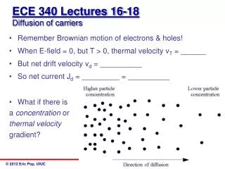
ECE 340 Lectures 16-18 Diffusion of carriers. Remember Brownian motion of electrons & holes! When E-field = 0, but T > 0, thermal velocity v T = ______ But net drift velocity v d = __________ So net current J d = _________ = __________ What if there is a concentration or

E N D
ECE 340 Lectures 16-18Diffusion of carriers • Remember Brownian motion of electrons & holes! • When E-field = 0, but T > 0, thermal velocity vT = ______ • But net drift velocity vd = __________ • So net current Jd = _________ = __________ • What if there is a concentration or thermal velocity gradient?
Is there a net flux of particles? Is there a net current? • Examples of diffusion: • ___________ • ___________ • ___________ • One-dimensional diffusion example:
How would you set up diffusion in a semiconductor? You need something to drive it out of equilibrium. • What drives the net diffusion current? The concentration gradients! (no n or p gradient, no net current)
Mathematically: • JN,diff = • JP,diff = • Where DN and DP are the diffusion coefficients or diffusivity • Now, we can FINALLY write down the TOTAL currents… • For electrons: • For holes: • And TOTAL current:
Interesting point: minority carriers contribute little to drift current (usually, too few of them!), BUT if their gradient is high enough… • Under equilibrium, open-circuit conditions, the total current must always be = • I.e. Jdrift = - Jdiffusion • More mathematically, for electrons: • So any disturbance (e.g. light, doping gradient, thermal gradient) which may set up a carrier concentration gradient, will also internally set up a built-in __________________
What is the relationship between mobility and diffusivity? • Consider this band diagram: • Going back to drift + diffusion = 0 in equilibrium:
Leads us to the Einstein Relationship: • This is very, very important because it connects diffusivity with mobility, which we already know how to look up. Plus, it rhymes in many languages so it’s easy to remember. • The Einstein Relationship (almost) always holds true.
Ex: The hole density in an n-type silicon wafer (ND = 1017 cm-3) decreases linearly from 1014 cm-3 to 1013 cm-3 between x = 0 and x = 1 μm (why?). Calculate the hole diffusion current.
Let’s recap the simple diffusion lessons so far: • Diffusion without recombination (driven by dn/dx) • Einstein relationship (D/μ = kT/q) • kT/q at room temperature ~ 0.026 V (this is worth memorizing, but be careful at temperatures different from 300 K) • Mobility μ look up in tables, then get diffusivity (be careful with total background doping concentration, NA+ND) • Next we examine: • Diffusion with recombination • The diffusion length (distance until they recombine)
Assume holes (p) are minority carriers • Consider simple volume element where we have both generation, recombination, and holes passing through due to a concentration gradient (dp/dx) • Simple “bean counting” in the little volume • Rate of “bean” or “bubble” population increase = (current IN – current OUT) – bean recombination
Note, this technique is very powerful (and often used) in any Finite Element (FE) computational or mathematical model. • So let’s count “beans” (“bubbles”): • Recombination rate = # excess bubbles (δp) / recombination time (τ) • Current (#bubbles) IN – Current (#bubbles) OUT = JIN – JOUT / dx • Note units (VERY important check): • Bubble current is bubbles/cm2/s, but bubble rate of change (G&R) is bubbles/cm3/s • So, must account for width (dx ~ cm) of volume slice • Why does the first equality hold? (simple, boring math…)
Why is there a (diffusion) current derivative divided by q? • Of course, e.g. for holes: so, • So the diffusion equation (which is just a special case of the continuity equation above) becomes: • This allows us to solve for the minority carrier concentrations in space and time (here, holes)
Note, this is applicable only to minority carriers, whose net motion is entirely dominated by diffusion (gradients) • What does this mean in steady-state? • The diffusion equation in steady-state: • Interesting: this is what a lot of other diffusion problems look like in steady-state. Other examples? • The diffusion length Lp = _________ is a figure of merit.
Consider an example under steady-state illumination: • Solve diffusion equation: δp(x) = Δpe-x/Lp
Plot: • Physically, the diffusion lengths (Lp and Ln) are the average distance that minority carriers can diffuse into a sea of majority carriers before being annihilated (recombining). • What devices is this useful in?! (peek ahead)
Ex:A) Calculate minority carrier diffusion length in silicon with ND = 1016 cm-3 and τp = 1 μs. B) Assuming 1015 cm-3 excess holes photogenerated at the surface, what is the diffusion current at 1 μm depth?