Download
1 / 66
660 likes | 869 Vues
Seismic Waves and Inversion Vandana Chopra Eddie Willett Ben Schrooten Shawn Borchardt. Topics. What are Seismic Waves??????? History Types of Seismic Waves. What are Seismic Waves ???. Seismic waves are the vibrations from earthquakes that travel through the Earth

E N D
Seismic Waves and Inversion • Vandana Chopra • Eddie Willett • Ben Schrooten • Shawn Borchardt
Topics • What are Seismic Waves??????? • History • Types of Seismic Waves
What are Seismic Waves ??? • Seismic waves are the vibrations from earthquakes that travel through the Earth • They are the waves of energy suddenly created by the breaking up of rock within the earth or an explosion .They are the energy that travels through the earth and is recorded on seismographs
History • Seismology - the Study of Earthquakes and Seismic Waves • 1) Dates back almost 2000 years
History Cont • Around 132 AD, Chinese scientist Chang Heng invented the first seismoscope, an instrument that could register the occurrence of an earthquake. • They are recorded on instruments called seismographs. Seismographs record a zigzag trace that shows the varying amplitude of ground oscillations beneath the instrument. Sensitive seismographs, which greatly magnify these ground motions, can detect strong earthquakes from sources anywhere in the world. The time, location and magnitude of an earthquake can be determined from the data recorded by seismograph stations.
Seismometers and Seismographs • Seismometers are instruments for detecting ground motions • Seismographs are instruments for recording seismic waves from earthquakes. • Seismometers are based on the principal of an “inertial mass” • Seismographs amplify, record, and display the seismic waves • Recordings are called seismograms
Types of Seismic Waves • Body wavesTravel through the earth's interior • Surface Waves Travel along the earth's surface - similar to ocean waves
P-Wave(Body Wave) Primary or compressional (P) waves a) The first kind of body wave is the P wave or primary wave. This is the fastest kind of seismic wave. b) The P wave can move through solid rock and fluids, like water or the liquid layers of the earth. c) It pushes and pulls the rock it moves through just like sound waves push and pull the air. d) Highest velocity (6 km/sec in the crust)
Secondary Wave (S Wave) • Secondary or shear (S) wavesa)The second type of body wave is the S wave or secondary wave, which is the second wave you feel in an earthquake. • b) An S wave is slower than a P wave and can only move through solid rock. (3.6 km/sec in the crust) • c) This wave moves rock up and down, or side-to-side.
L-Wave • Love Waves • The first kind of surface wave is called a Love wave, named after A.E.H. Love, a British mathematician who worked out the mathematical model for this kind of wave in 1911. • It's the fastest surface wave and moves the ground from side-to-side.
Rayleigh Waves • Rayleigh Waves • The other kind of surface wave is the Rayleigh wave, named for John William Strutt, Lord Rayleigh, who mathematically predicted the existence of this kind of wave in 1885. • A Rayleigh wave rolls along the ground just like a wave rolls across a lake or an ocean. Because it rolls, it moves the ground up and down, and side-to-side in the same direction that the wave is moving. • Most of the shaking felt from an earthquake is due to the Rayleigh wave, which can be much larger than the other waves.
Outline I’m going to briefly cover three different Seismic wave equations -Inhomogeneous Constant Density 2-D Wave Equation -First Order Wave Equation -Acoustic Wave Equation and how it’s derived
Inhomogeneous Constant Density 2-D Wave Equation The pressure wave field is ψ and the seismic source is src(t) Media velocity, C(x,z), the sound speed with x being the surface coordinate and z being the depth coordinate
First Order Wave Equation Again the pressure wave field is ψ, the sound speed is c and x is the surface coordinate Parameter α is determines the propagation direction of the wave This is the simplest wave propagation model
Wave Equation Variables • Mass and Momentum are conserved (basis for development of wave equation) • Mass density is ρ • Particle velocity is ψ • Fluid Pressure is P • Three spatial coordinates xi (i=1,2,3) for domain Ω • Stress matrix is σij (stress within the fluid)
Conservation of Mass and Momentum Momentum Stress matrix Kronecker delta function (pseudotensor) Mass
Some Considerations Considering small perturbations Δ in Particle velocity Density Pressure And with Euler’s Equation with the viscosity equal to zero And realizing P0 is constant and fb is negligible we have
Derivations The initial medium is at rest so Euler’s Equation can be changed to eliminating the substantial derivatives. Then we let the gradient of Φ be equal to the particle velocity giving us
Derivations cont. Next we assume the derivatives of space and time can be changed therefore And removing the gradient operator on both sides gives us Now the compressibility C and bulk modulus of K are defined in terms of a unit volume V and ΔV
Derivations cont. The change in the change of fluid pressure P is now Now computing the derivative of this equation with respect to time is showing that the change in pressure is related to the change in density. Then substitutions with this equation gives us
Derivations cont. Now using the conservation of mass equation with the previous equation and time derivative gives us Then using the time derivative again we get And finally…
Derivations Concluded We have the Acoustic Wave Equation where is the speed of sound in the medium
Sources • Seismic Wave Propagation Modeling and Inversion www.math.fu-berlin.de/serv/comp/tutorials/csep • www.llnl.gov/liv_comp/meiko/apps/larsen/larsen3.gif
Reasons for Computational methods in Seismology • Computer development • More memory • 64k most accessible for single point • Early 1970’s rule of thumb • 1k for 1K of computer memory • Used more in the field • Size shrank explosively from 1960’s – 1990’s • Data acquisition, processing, and telemetry • Processing speed increase
Seismic Station coverage • Worldwide coverage by a single network of computers • good azimuthal and fair to good depth control for major earthquakes • Brought about software to analyze the data on this network
Early computer based study • Dorman & Ewing surface-wave data inversion in 1962 • earthquake location by Bolt, 1960; Flinn, 1960; Nordquist, 1962; Eaton, 1969) • Jerry Eaton first to include source code for his program • Credited with opening up software development to others • Computed travel times and derivatives for a source inside multiple layers over a half space.
Developments in the 80’s • Many groups compiled algorithms • Methods in Computational Physics • the two volumes of“Computer Programs in Earthquake Seismology” • Other computer code algorithms were also published in the engineering and geophysics literature
Developments up until today • A Working Group on Personal Computers in Seismicity Studies was created in 1994 • todays personal computers are taking the place of mainframes in this field • This has been the trend since 1980’s • The publication and distribution of seismological software is a major focus
Software packages available • Here are a few • CWP/SU: Seismic Unix: The Instant Seismic Processing and Research Environment • GeoFEM A multi-purpose / multi-physics parallel finite element solver for the solid earth.
Earthquakes Seismological activity as of 4/4/2002 11:21 AM
Software • Seismic Waves: A program for the visualization of wave propagation • By Antonello Trova • http://www.dicea.unifi.it/gfis/didattica.html
References and more info • http://www.iris.washington.edu/DOCS/off_software.htm • http://orfeus.knmi.nl/other.services/software.links.shtml • http://www.dicea.unifi.it/gfis/didattica.html • http://www-gpi.physik.uni-karlsruhe.de/pub/martin/MPS/ • http://wwwrses.anu.edu.au/seismology/ar98/swp.html • http://www.nea.fr/abs/html/ests1300.html • http://www.cwp.mines.edu/software.html • http://www.iris.washington.edu/seismic/60_2040_1_8.html • http://www.es.ucsc.edu/~smf/research.html • http://nisee.berkeley.edu/ • http://www.seismo.unr.edu/ftp/pub/louie/class/100/seismic-waves.html • http://mvhs1.mbhs.edu/mvhsproj/Earthquake/eq.html • http://www.riken.go.jp/lab-www/CHIKAKU/index-e.html(found it interesting, but cannot read Japanese) • http://www.cs.arizona.edu/japan/www/atip/public/atip.reports.99/atip99.043.html • http://www.engr.usask.ca/~macphed/finite/fe_resources/node162.html
Seismic Wave Projects And Visualizations Talking Team #2
Why are seismic waves important? Some things seismic waves are good for include ·Mapping the Interior of the Earth ·Monitoring the Compliance of the Comprehensive Test Ban Treaty ·Detection of Contaminated Aquifers ·Finding Prospective Oil and Natural Gas Locations
http://www.mines.edu/fs_home/tboyd/GP311/MODULES/SEIS/NOTES/Lmovie.htmlhttp://www.mines.edu/fs_home/tboyd/GP311/MODULES/SEIS/NOTES/Lmovie.html ·We Collect Information from the waves as they are reflected back to us and as they propagate to the other ends of the medium. ·What would happen if there was only 1 medium?
The P and S wave velocities of various earth materials are shown below. Material P wave Velocity (m/s) S wave Velocity (m/s) Air 332 Water 1400-1500 Petroleum 1300-1400 Steel 6100 3500 Concrete 3600 2000 Granite 5500-5900 2800-3000 Basalt 6400 3200 Sandstone 1400-4300 700-2800 Limestone 5900-6100 2800-3000 Sand (Unsaturated) 200-1000 80-400 Sand (Saturated) 800-2200 320-880 Clay 1000-2500 400-1000 Glacial Till (Saturated) 1500-2500 600-1000 The P and S wave velocities of various earth materials are shown below.
Visualizations Done With Seismic Wave Data in Supercomputing 3-D Seismic Wave Propagation on a Global and Regional Scale: Earthquakes, Fault Zones, Volcanoes Information and Images Source: Prof. Dr. Heiner Igel Institute of Geophysics, Ludwig-Maximilians-University, Germany Whats the purpose of the accurate simulation of seismic wave propagation through realistic 3-D Earth Models? ·Further understanding of the dynamic behavior of our planet ·Deterministic earthquake fore-casting, assessing risks for various zones (i.e. San Francisco Bay Area) ·Understanding active volcanic areas for risk assessment
Goals of the project: 1.Parallelization and implementation of algorithms for numerical wave propagation on the Hitachi SR8000-F1 2.Verification of the codes and analysis of their efficiency 3.First applications to realistic problems Before moving into 3-D the base numerical solutions had to be compared to analytical solutions for simple (layered) model geometries.
The System used for Simulation ·Hitachi SR-8000 F1 ·Typical Speed 750Mflops per node ·Internode Transfer Speed 1GB/s Technical Methods ·Numerical solutions to the elastic wave equations in Cartesian and spherical coordinates. ·Time dependent partial differential equations are solved numerically using high-order finite difference methods ·Space-dependent fields are defined on a 3-D grid and the time extrapolation is carried out using a Taylor expansion ·Space derivatives are calculated by explicit high-order finite-difference schemes that do not necessitate the use of matrix inversion techniques Languages Used ·Fortran 90 coupled with the Message Passing Interface (MPI)