Download
1 / 1
20 likes | 139 Vues
Table 1: correlation matrix and VIF for all the variables. Dependent Variable. Independent Variable. Corr. Value. p-Value. VIF. AREA. October Band 1. -0.036. 0.533. ----------. Variables. Parameter estimate. VIF. Variables. Parameter estimate. VIF. (a). AREA.

E N D
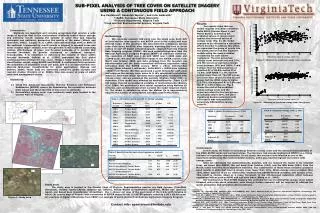
Table 1: correlation matrix and VIF for all the variables Dependent Variable Independent Variable Corr. Value p-Value VIF AREA October Band 1 -0.036 0.533 ---------- Variables Parameter estimate VIF Variables Parameter estimate VIF (a) AREA October Band 2 -0.360 < .0001 2.79 AREA October Band 3 -0.153 0.007 8.54 Intercept 151.75 0.00 Intercept 81.71 0.00 AREA March Band 1 0.193 < .0001 137.30 (b) OB2 -119.07 1.23 OB2 -91.39 1.57 AREA March Band 2 0.001 0.983 ---------- MB3 -141.26 1.19 MB3 51.04 1.31 AREA March Band 3 -0.109 0.052 15.91 DNDVI 1.64 1.09 DNDVI 2.21 1.37 AREA DNDVI 0.371 < .0001 1.95 R2 0.04 AREA March Brightness -0.211 < .0001 5322.49 R2 0.72 Adjusted- R2 0.03 Adjusted- R2 0.69 (c) AREA March Greenness -0.235 < .0001 2269.00 RMSE 19.79 RMSE 2.73 AREA March Wetness 0.254 < .0001 8886.99 AREA October Brightness -0.263 < .0001 7.46 AREA October Greenness -0.020 0.730 ---------- AREA October Wetness 0.092 0.109 ---------- Table 2: Results from the best subset regression analysis Variables in model R2 Adj-R2 Cp RMSE DNDVI 0.13 0.13 37.89 23.60 DNDVI, October Brightness 0.23 0.22 6.84 22.33 DNDVI, March Band 3, October Band 2 0.23 0.22 4.32 22.31 DNDVI, March Band 3, October Band 2, October Brightness 0.24 0.23 4.34 22.27 (e) DNDVI, March Band 3, October Band 2, October Band 3, October Brightness 0.24 0.22 6.00 22.29 (d) SUB-PIXEL ANALYSIS OF TREE COVER ON SATELLITE IMAGERY USING A CONTINUOUS FIELD APPROACH Eva Pantaleoni¥, Randolph Wynne‡, , and John Galbraith* ¥IAgER, Tennessee State University ‡Forestry Department, Virginia Tech *Crop and Soil Environmental Science, Virginia Tech Results: Our results show that our model requires only three variables: Delta NDVI, October Band 2, and March Band 3. Examining the predicted values of canopy cover against the observed values of canopy cover (Fig. 2), the model appears to be affected by a saturation effect. In order to address this effect, we separated the group of points into two parts, and we ran two separate models using the same variables selected by the best subset regression. The first group had canopy cover between zero and 15%, and the second group had a canopy cover between 16% and 100%. Table 3 shows that the first group has an adjusted-R2 of 69.0% and an R2 of 72.0%, with RMSE = 2.7% and VIF values lower than 10. The VIF values are lower than 10 also for the second group, but the RMSE value is higher (13.7%), the adjusted-R2 is 3.0% and the R2 is 4.0% (Table 4). Fig. 3 shows the plot of the predicted values canopy cover and the observed values for the two groups. At canopies above 15%, the pixel signatures became saturated with color and it was not possible to accurately differentiate canopy cover%. • Introduction: • Wetlands are important and complex ecosystems that provide a wide range of services vital to the environment. Wetlands control water storage and indirectly runoff, slowing the velocity of water flow and trapping sediments and nutrients, preserving the quality of the water (Mitsch and Gosselink, 1993). Cooper et al. (1987) demonstrated that 85% to 90% of the sediment transported by runoff events is trapped in wooded areas and never reaches major streams. Even though there is still a debate concerning relative effectiveness of grass and forested wetlands, it is evident that forested wetlands do provide resistance to sediment transport. Consequently, it is important to determine the density of trees within forested wetlands.DeFries et al. (2000) generated the first global continuous field product for tree cover, fitting a linear mixture model to a classification output, using AVHRR and MODIS. A continuous field represents the proportion of vegetation cover per pixel, and it is an improvement over discrete land-cover classifications for some applications (Hansen and DeFries, 2004). These data are extremely useful for global analysis and regional studies (Franklin et al. 2000), they lose power at scale at which most land management occurs. • Objectives: • Using the Advanced Spaceborne Thermal Emission and Reflection Radiometer (ASTER) sensor for determining the correlation between pixel values and the proportion of tree cover in wetlands. • Determining canopy cover over extremely small plots located in the Coastal Plain of Virginia. Methodology: We randomly selected 300 plots over the study area. Each 225 m2 plot had the area equal to one ASTER pixel in the visible and near infrared range of the spectrum. We calculated the continuous canopy cover field using ArcGIS® after manually digitizing the tree or shrub outline on leaf-off digital orthophotographs obtained from the Virginia Base Mapping program (VBMP). We used aerial photographs from the National Agriculture Imagery Program (NAIP) as additional reference. The resolution of NAIP was 1 m, and VBMP was 1:4800 scale and 1:2400 scale. We used the first three bands of two ASTER scenes, from March and October 2005, and data obtained from the tasseled cap transformation and the delta normalized difference vegetation index calculated from the ASTER scenes. NDVI = (Near Infrared-Red bands)/(Near infrared + red bands). Delta NDVI = (NDVI from October – NDVI from March).We then generated a point feature for each pixel and assigned the canopy cover value to it. We calculated a correlation matrix to determine which variables were significantly correlated with canopy cover, and we examined the variable inflation factor (VIF) to determine if the model was affected by multicollinearity (Table 1). A VIF higher than 10 is considered evidence of multicollinearity (Belsley et al. 1980). We performed a best subset regression using Mallows Cp criterion, and we determined which variable the model required (Table 2). The model is satisfactory when the Mallow Cp is approximately equal to the number of independent variables used in the model. Figure 2: Observed vs. predicted canopy cover, one group Figure 3: Observed vs. predicted canopy cover, two groups Table 4: results for canopy cover > 16% Table 3: results for canopy cover < 15% Conclusions: In this study, we found a relationship between canopy cover and the spectral characteristics of the VNIR ASTER bands and derived indices. The literature had already highlighted DNDVI as a strong indicator of vegetation characteristics. In our study, this measure was selected as one of the important variables by the model selection criteria, and it also had the highest correlation with canopy cover. After we addressed the multicollinearity problem, and we reduced the model to its simplest form, we found that DNDVI, the red band from October (OB2) and the NIR band (MB3) from the March scene were the most important variables. The combination of these three variables produces good results in plots that have a canopy cover lower than 16%. When canopy cover is higher than 15%, there appears to be no relationship between the ASTER-derived variables and canopy cover. This result is similar, albeit at a lower threshold, to the off-observed saturation effect between vegetation indices such as NDVI and leaf area index (Wang et al., 2005). Our conclusion is that ASTER imagery has potential for use in estimating canopy cover within forested and scrub-shrub wetlands, even though further research will be required to address the water absorption and saturation effect problems. Study area: The study area is located in the Coastal Plain of Virginia. Representative species are Bald Cypress (Taxodium distichum), Swamp Tupelo (Nyssa sylvatica var. biflora), Yellow Poplar (Liriodendrom tupilifera), Water Oak (Quercus nigra), and Sweet Gum (Liquidamber styraciflua). Fig. 1 shows: (a) map of the east coast of the U.S.A. with Virginia in black; (b) county map of Virginia with boundaries of ASTER scene in red; (c) ASTER granule covering a 60 x 60-km area; (d) example of digital orthophotos from VBMP; (e) example of aerial photos from National Agriculture Imagery Program. References: COOPER, J.R., GILLIAM, J.W., DANIELS, R.B., and ROBARGE, W.P., 1987, Riparian areas as filters for agricultural sediment. Proceedings, Soil Science Society of America, 51, 416-420. DEFRIES, RS, HANSEN, M.C., TOWNSHEND, J.R.G., 2000, Global continuous fields of vegetation characteristics: a linear mixture model applied to multi-year 8 km AVHRR data. International Journal of Remote Sensing, 21, 1389–414. FRANKLIN, J., WOODCOCK, C.E., AND WARBINGTON, R., 2000, Multi attribute Vegetation Maps of Forest Service Lands in California Supporting Resource Management Decisions. Photogrammetric Engineering & Remote Sensing, 66, 1209-1217. HANSEN, M.C., AND DEFRIES, R.S., 2004, Detecting Long-term Global Forest Change Using Continuous Fields of Tree-Cover Maps from 8-km Advanced Very High Resolution Radiometer (AVHRR) Data for the Years 1982-99. Ecosystems, 7, 695-716. MITSCH, W.J., and GOSSELINK, J.G., 1993, Wetlands. 2nd ed. (New York, NY: Van Nostrand Reinhold). WANG, Y., and SUN, D., 2005, The ASTER tasseled cap interactive transformation using Gramm-Schmidt method. MIPPR 2005: SAR and Multispectral Image processing, In Proceedings of the SPIE, 6043. Figure 1: study area Contact info: epantaleoni@tnstate.edu