Download
1 / 43
430 likes | 667 Vues
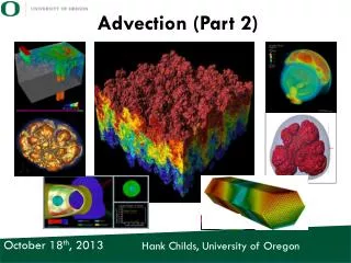
Advection (Part 2). Hank Childs, University of Oregon. October 18 th , 2013. Announcements. Bonus OH Mon 1-2 Quiz on Weds Project #4 is out, due Mon. Today’s lecture: Review of advection Overview of project 4 More particle advection usages.

E N D
Advection (Part 2) Hank Childs, University of Oregon October 18th,2013
Announcements • Bonus OH Mon 1-2 • Quiz on Weds • Project #4 is out, due Mon. • Today’s lecture: • Review of advection • Overview of project 4 • More particle advection usages
From lecture #1: What should you do if you run into trouble? Start with Piazza Office Hours Email me: hank@cs.uoregon.edu
LERPing vectors X = B-A A B } t X A A+t*X • LERP = Linear Interpolate • Goal: interpolate vector between A and B. • Consider vector X, where X = B-A • A + t*(B-A) = A+t*X • Takeaway: • you can LERP the components individually • the above provides motivation for why this works
Overview of advection process • Place a massless particle at a seed location • Displace the particle according to the vector field • Result is an “integral curve” corresponding to the trajectory the particle travels • Math gets tricky
Formal definition for particle advection • Output is an integral curve, S, which follows trajectory of the advection • S(t) = position of curve at time t • S(t0) = p0 • t0: initial time • p0: initial position • S’(t) = v(t, S(t)) • v(t, p): velocity at time t and position p • S’(t): derivative of the integral curve at time t This is an ordinary differential equation (ODE).
The integral curve for particle advection is calculated iteratively S(t0) = p0 while (ShouldContinue()) { S(ti) = AdvanceStep(S(t(i-1)) } ShouldContinue(): keep stepping as long as it returns true How to do an advance?
AdvanceStep goal: to calculate Si from S(i-1) S0 S1 = AdvanceStep(S0) S4 = AdvanceStep(S3) S5= AdvanceStep(S4) S2 = AdvanceStep(S1) S3= AdvanceStep(S2) S1 S3 S4 S2 S5 This picture is misleading: steps are typically much smaller.
AdvanceStep Overview • Think of AdvanceStep as a function: • Input arguments: • S(i-1): Position, time • Output arguments: • Si: New position, new time (later than input time) • Optional input arguments: • More parameters to control the stepping process.
AdvanceStep Overview • Different numerical methods for implementing AdvanceStep: • Simplest version: Euler step • Most common: Runge-Kutta-4 (RK4) • Several others as well
Euler Method • Most basic method for solving an ODE • Idea: • First, choose step size: h. • Second,AdvanceStep(pi, ti) returns: • New position: pi+1 = pi+h*v(ti, pi) • New time: ti+1 = ti+h
Quiz Time: Euler Method • Euler Method: • New position: pi+1 = pi+h*v(ti, pi) • New time: ti+1 = ti+h • Let h=0.01s • Let p0 = (1,2,1) • Let t0 = 0s • Let v(p0, t0) = (-1, -2, -1) • What is (p1, t1) if you are using an Euler method? Answer: ((0.99, 1.98, 0.99), 0.01)
Runge-Kutta Method (RK4) • Most common method for solving an ODE • Definition: • First, choose step size, h. • Second,AdvanceStep(pi, ti) returns: • New position: pi+1 = pi+(1/6)*h*(k1+2k2+2k3+k4) • k1 = v(ti, pi) • k2 = v(ti + h/2, pi + h/2*k1) • k3= v(ti + h/2, pi + h/2*k2) • k4= v(ti + h, pi + h*k3) • New time: ti+1 = ti+h
Physical interpretation of RK4 • New position: pi+1 = pi+(1/6)*h*(k1+2k2+2k3+k4) • k1 = v(ti, pi) • k2 = v(ti + h/2, pi + h/2*k1) • k3= v(ti + h/2, pi + h/2*k2) • k4= v(ti + h, pi + h*k3) v(ti+h, pi+h*k3) = k4 pi pi+ h/2*k2 pi+ h*k3 v(ti+h/2, pi+h/2*k2) = k3 v(ti, pi) = k1 pi+ h/2*k1 v(ti+h/2, pi+h/2*k1) = k2 Evaluate 4 velocities, use combination to calculate pi+1
Reminder • Omitting review of material in Lecture #5 on errors in advection step.
Termination causes Quiz: which one is time and which one is distance? • Criteria reached • Time • Distance • Number of steps • Same as time? • Other advanced criteria, based on particle advection purpose • Can’t meet criteria • Exit the volume • Advect into a sink Distance Time
Steady versus Unsteady State • Unsteady state: the velocity field evolves over time • Steady state: the velocity field has reached steady state and remains unchanged as time evolves
Most common particle advection technique: streamlines and pathlines • Idea: plot the entire trajectory of the particle all at one time. Streamlines in the “fish tank”
Streamline vsPathlines • Streamlines: plot trajectory of a particle from a steady state field • Pathlines: plot trajectory of a particle from an unsteady state field • Quiz: most common configuration? • Neither!! • Pretend an unsteady state field is actually steady state and plot streamlines from one moment in time. • Quiz: why would anyone want to do this? • (answer: performance)
Lots more to talk about • How do we pragmatically deal with unsteady state flow (velocities that change over time)? • More operations based on particle advection • Stability of results • You all will figure this out (project 5)
Dealing with steady state velocities • Euler Method (unsteady): • New position: pi+1 = pi+h*v(ti, pi) • New time: ti+1 = ti+h • Euler Method (steady): • New position: pi+1 = pi+h*v(t0, pi) • New time: ti+1 = ti+h
Unsteady vs Steady: RK4 • Unsteady: • New position: pi+1 = pi+(1/6)*h*(k1+2k2+2k3+k4) • k1 = v(ti, pi) • k2 = v(ti + h/2, pi + h/2*k1) • k3= v(ti + h/2, pi + h/2*k2) • k4= v(ti + h, pi + h*k3) • New time: ti+1 = ti+h
Unsteady vs Steady: RK4 • Steady: • New position: pi+1 = pi+(1/6)*h*(k1+2k2+2k3+k4) • k1 = v(t0, pi) • k2 = v(t0, pi + h/2*k1) • k3= v(t0, pi + h/2*k2) • k4= v(t0, pi + h*k3) • New time: ti+1 = ti+h
Project 4 • Assigned October 16th, prompt online • Due October 21st, midnight ( October 22nd, 6am) • Worth 7% of your grade • Provide: • Code skeleton online • Correct answers provided • You send me: • source code • screenshot with: • text output on screen • image of results
Project 4 in a nutshell • Do some vector LERPing • Do particle advection with Euler steps • Examine results
Project 4 in a nutshell • Implement 3 methods: • EvaluateVectorFieldAtLocation • LERP vector field. (Reuse code from before, but now multiple component) • AdvectWithEulerStep • You know how to do this • CalculateArcLength • What is the total length of the resulting trajectory?
Project 5 in a nutshell • Implement Runge-Kutta 4 • Assess the quality of RK4 vs Euler • Open ended project • I don’t tell you how to do this assessment. • You will need to figure it out. • Multiple right answers • Deliverable: short report (~1 page) describing your conclusions and methodology. • Pretend that your boss wants to know which method to use and you have to convince her which one is the best and why. • Not everyone will receive full credit.
Additional Particle Advection Techniques • This content courtesy of Christoph Garth, Kaiserslautern University.
Streamline, Pathline,Timeline, Streakline, • Streamline: steady state velocity, plot trajectory of a curve • Pathline: unsteady state velocity, plot trajectory of a curve • Timeline: start with a line, advect that line and plot the line’s position at some future time
Time Surface • Advect a surface and see where it goes • “A sheet blowing in the wind”
Streamline, Pathline,Timeline, Streakline • Streamline: steady state velocity, plot trajectory of a curve • Pathline: unsteady state velocity, plot trajectory of a curve • Timeline: start with a line, advect that line and plot the line’s position at some future time • Streakline: unsteady state, introduce new particles at a location continuously
Streaklines Will do an example on the board
Stream surface: • Start with a seeding curve • Advect the curve to form a surface
Stream surface: • Start with a seeding curve • Advect the curve to form a surface
Stream Surface Computation • Skeleton from Integral Curves + Timelines
Stream Surface Computation • Skeleton from Integral Curves + Timelines • Triangulation Generation of Accurate Integral Surfaces in Time-Dependent Vector Fields. C. Garth, H. Krishnan, X. Tricoche, T. Bobach, K. I. Joy. In IEEE TVCG, 14(6):1404–1411, 2007
Stream Surface Example #2 Vortex system behind ellipsoid
Lagrangian Methods • Visualize manifolds of maximal stretching in a flow, as indicated by dense particles • Finite-Time Lyapunov Exponent (FTLE) www.vacet.org
Lagrangian Methods • Visualize manifolds of maximal stretching in a flow, as indicated by dense particles • forward in time: FTLE+ indicates divergence • Backward in time: FTLE+ indicates convergence www.vacet.org