Download
1 / 15
150 likes | 353 Vues
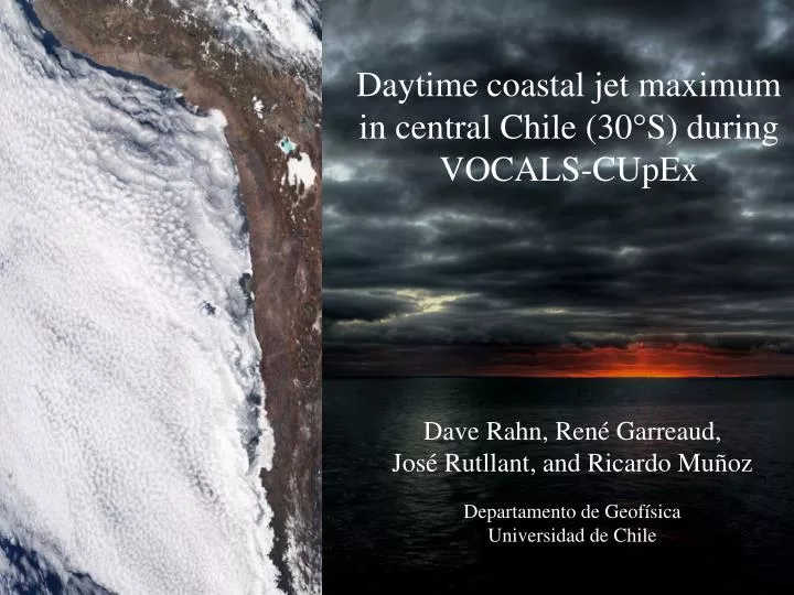
Daytime coastal jet maximum in central Chile (30°S) during VOCALS- CUpEx. Dave Rahn, René Garreaud, José Rutllant , and Ricardo Muñoz Departamento de Geofísica Universidad de Chile. Field Campaign. VOCALS - Chilean Upwelling Experiment ( CUpEx )

E N D
Daytime coastal jet maximum in central Chile (30°S) during VOCALS-CUpEx Dave Rahn, René Garreaud, José Rutllant, and Ricardo Muñoz Departamento de Geofísica Universidad de Chile
Field Campaign • VOCALS - Chilean Upwelling Experiment (CUpEx) • A vast amount of data in a previously data-void region: • Buoy, Ship, Aircraft, Land stations, Radiosonde, Remote Sensing • High resolution numerical simulations. • More details in Garreaud’s talk.
Coastal Jet • High wind extends a few hundred kilometers offshore centered around 30°S. • Subsequent analysis is valid for the 8-day high wind period: • 25 Nov. – 3 Dec. ASCAT 10-m winds (m s-1) during the high wind period. 5-minute averaged wind speed (m s-1) at Talcaruca during the intensive phase of the field campaign. Shaded regions indicate low-wind periods.
Fluid System • Marine Atmospheric Boundary Layer (MBL) • Cool, well-mixed layer near the surface • Capped by temperature inversion • MBL next to coastal mountains allows for a general two layer fluid system with a lateral boundary, supporting a variety of features: • Coastal Jet • Coastal Upwelling • Barrier Jet • Trapped density currents • Topographically trapped ageostrophic response • Kelvin waves • Hydraulic effects often used to describe features linked to topography.
Numerical Simulation • Weather and Research Forecasting (WRF, v3.1.1) model. • Global Forecast System (GFS) analyses (1°x1°) for initialization/B.C.’s • 0000 UTC 20 October 2009 to 0000 UTC 6 December 2009 • Mother Domain: 9 km • Inner Domain: 3 km • Vertical Levels: 56 sigma • ~60 m at 1 km • ~100 m at 2 km • Parameters: Thompson microphysics, rapid radiative transfer model for longwave radiation, Dudhia for shortwave radiation, Monin-Obukhov (Janjic) surface scheme, Pleim land-surface model, Mellor-Yamada-Janjic boundary layer scheme, Betts-Miller-Janjic cumulus scheme, second order turbulence and mixing, and a horizontal Smagorinsky first-order closure eddy coefficient.
WEST EAST Zonal cross section Left: Meridional wind speed (m s-1, color), in-the-plane (u, z) vectors (m s-1), and potential temperature (K, contours) along 30°S (terrain at 30.4°S depicted by transparent green silhouette) at (a) 1200 UTC and (b) 2100 UTC. (c) 2100 – 1200 UTC potential temperature difference (K, color), meridional difference (m s-1, contours), and in-the-plane (u,z) vector difference (m s-1).
SOUTH NORTH Meridional cross section • Place holder Left: Zonal wind speed (m s-1, color), in-the-plane (v, z) vectors (m s-1), and potential temperature (K, contours) along 71.6°W at (d) 1200 UTC and (e) 2100 UTC. (f) 2100 – 1200 UTC potential temperature difference (K, color), meridional difference (m s-1, contours), and in-the-plane (v,z) vector difference (m s-1).
Pressure response • Over Tongoy Bay, afternoon surface pressure drops rapidly in the bay under the warming temperatures. • Offshore, changes in temperature and surface pressure is small. • Resulting in a large localized gradient along coastal range axis. Above: Average diurnal temperature difference. • While there are model differences, resulting surface pressure drop is the same. Right: The average temperature (°C, color) and surface pressure (hPa, contours).
Diurnal pressure differences • Data from high wind period. • Mean removed from model and observations from both station to remove offsets. • Range and diurnal cycle of observations and model agree well. • Discrepancy at 0900 UTC, local effect? • From 12 UTC to 21 UTC pressure difference decreases 1.3 hPa indicating pressure drops faster in TGY. • Remaining 0.3 hPa from diurnal tide.
Ageostropic Wind (1) (2) Va: Ageostrophic wind f : Coriolis Parameter Vg: Geostrophic Wind Advective Component Isallobaric Component • Placeholder Rahn and Parish 2007
Summary • Local 10-m wind maximum in the afternoon extending ~60 km north. • Why? • Small MBL/Temp. changes offshore • Large changes over the bay • Warm air advected over Tongoy Bay from the valley to the south. • Strong baroclinic zone localized close to LdV. • Large pressure gradient results • Topography sensitivity suggests that maximum would exist regardless. • Coastal range acts to enhance the local gradient.
Recapping the Highlights… • Coastal Jet at Lengua de Vaca Questions? • Ongoing work… • Surface stations continue to record data • Aircraft measurements along the coast. http://www.dgf.uchile.cl/~darahn/
Synoptic Summary • While the vertical velocity and residual tend to be the dominant opposing terms, change of MBL depth appears to be tied closely to the variability in advection. • Extent of the synoptic influence from the mid-latitudes is shown and can greatly impact the subtropical region. • Generalization of these findings requires analysis over much longer/different time periods. • Ongoing work… • More detailed work on MBL characteristics under strong synoptic forcing (i.e., how fast it can recover, how exactly does it recover). • Additional work on marine cyclogenesis and interaction with the MBL as well as the effects translated into the subtropics.
Right: Time series at Talcaruca depicting potential temperature (contours, K) and wind components (color, m s-1) for afternoon soundings only. Bottom: Average profiles of potential temperature (K) and wind in the morning (top) and afternoon (below) 25 Nov -3 Dec.