Download
1 / 49
560 likes | 788 Vues
SAMPLING DISTRIBUTION OF MEANS & PROPORTIONS. SAMPLING AND SAMPLING VARIATION. Sample Knowledge of students No. of red blood cells in a person Length of the life of electric bulbs Population Population census– whole population.

E N D
SAMPLING AND SAMPLING VARIATION Sample Knowledge of students No. of red blood cells in a person Length of the life of electric bulbs Population Population census– whole population
Repeat the same study, under exactly similar conditions, we will not necessarily get identical results. • Example: In a clinical trail of 200 patients we find that the efficacy of a particular drug is 75% If we repeat the study using the same drug in another group of similar 200 patients we will not get the same efficacy of 75%. It could be 78% or 71%. “Different results from different trails though all of them conducted under the same conditions”
Example: • If the two drugs have the same efficacy then the difference between the cure rates with these two drugs should be zero. • But in practice we may not get a difference of zero. • If we find the difference is small say 2%, 3%, or 5%, we may accept the hypothesis that the two drugs are equally effective. • On the other hand, if we find the difference to be large say 25%, we would infer that the difference is very large and conclude that the drugs are not of equally efficacy.
Example:If we testing the claim of pharmaceutical company that the efficacy of a particular drug is 80%. We may accept the company’s claim if we observe the efficacy in the trail to be 78%, 81%, 83% or 77%. But if the efficacy in trail happens to be 50%, we would have good cause to feel that true efficacy cannot be 80%. And the chance of such happening must be very low. We then tend to dismiss the claim that the efficacy of the drug is 80%.
THEREFORE “WHILE TAKING DECISIONS BASED ON EXPERIMENTAL DATA WE MUST GIVE SOME ALLOWANCE FOR SAMPLING VARIATION “. “VARIATION BETWEEN ONE SAMPLE AND ANOTHER SAMPLE IS KNOWN AS SAMPLING VARIATION”.
Inference – extension of results obtained from an experiment (sample) to the general population • use of sample data to draw conclusions about entire population • Parameter – number that describes a population • Value is not usually known • We are unable to examine population • Statistic – number computed from sample data • Estimate unknown parameters • Computed to estimate unknown parameters • Mean, standard deviation, variability, etc.. Notations population mean sample mean
= Population mean • Sample mean is a random variable. • If the sample was randomly drawn, then any differences between the obtained sample mean and the true population mean is due to sampling error. • Any difference between and μ is due to the fact that different people show up in different samples • If is not equal to μ , the difference is due to sampling error. • “Sampling error” is normal, it isto-be-expected variability of samples
How can experimental results be trusted? If is rarely exactly right and varies from sample to sample, why is it not a reasonable estimate of the population mean μ? • How can we describe the behavior of the statistics from different samples? • E.g. the mean value
Very rarely do sample values coincide with the population value (parameter). The discrepancy between the sample value and the parameter is known as sampling error, when this discrepancy is the result of random sampling. Fortunately, these errors behave systematically and have a characteristic distribution.
SAMPLING DISTRIBUTIONThe sample distribution is the distribution of all possible sample means that could be drawn from the population.
SAMPLING DISTRIBUTIONS What would happen if we took many samples of 10 subjects from the population? • Steps: • Take a large number of samples of size 10 from the population • Calculate the sample mean for each sample • Make a histogram of the mean values • Examine the distribution displayed in the histogram for shape, center, and spread, as well as outliers and other deviations
A sample of 3 students from a class – a population of 6 students and measure students GPA
Draw each possible sample from this ‘population’: Karen 2.6 Susan 2.1 Bill 2.3 Calvin 1.2 David 2.4 Rose 3.0
With samples of n = 3 from this population of N = 6 there are 20 different sample possibilities:
Note that every different sample would produce a different mean and s.d., ONE SAMPLE = Susan + Karen +Bill / 3 = 2.1+2.6+2.3 / 3 = 7.0 / 3 = 2.3 Standard Deviation: (2.1-2.3) 2 = .22 = .04 (2.6-2.3) 2 = .32 = .09 (2.3-2.3) 2 = 02 = 0 s2=.13/3 and s = =.21 So this one sample of 3 has a mean of 2.3 and a sd of .21
What about other samples? • A SECOND SAMPLE = Susan + Karen + Calvin = 2.1 + 2.6 + 1.2 = 1.97 SD = .58 • 20th SAMPLE = Karen + Rose + David = 2.6 + 3.0 + 2.4 = 2.67 SD = .25
Assume the true mean of the population is known, in this simple case of 6 people and can be calculated as 13.6/6 = =2.27 • The mean of the sampling distribution (i.e., the mean of all 20 samples) is 2.30.
What is a Sampling Distribution? • A distribution made up of every conceivable sample drawn from a population. • A sampling distribution is almost always a hypothetical distribution because typically you do not have and cannot calculate every conceivable sample mean. • The mean of the sampling distribution is an unbiased estimator of the population mean with a computable standard deviation.
LAW OF LARGE NUMBERS 1) If we keep taking larger and larger samples, the statistic is guaranteed to get closer and closer to the parameter value.
N = 1 N = 2 N = 25 N = 10
Central Limit Theorem If all possible random samples, each the size of your sample, were taken from any population then the sampling distribution of sample means will have: • a mean equal to the population mean • a standard deviation equal to The sampling distribution will be normally distributed IF EITHER: • the parent population from which you are sampling is normally distributed OR • IF the sample size is greater than n=30.
ILLUSTRATION OF SAMPLING DISTRIBUTIONS Draw 500 different SRSs. What happens to the shape of the sampling distribution as the size of the sample increases?
Key Observations • As the sample size increases the mean of the sampling distribution comes to more closely approximate the true population mean, here known to be m = 3.5 • AND-this critical-the standard error-that is the standard deviation of the sampling distribution – gets systematically narrower.
Three main pointsabout sampling distributions • Probabilistically, as the sample size gets bigger the sampling distribution better approximates a normal distribution. • The mean of the sampling distribution will more closely estimate the population parameter as the sample size increases. • The standard error (SE) gets narrower and narrower as the sample size increases. Thus, we will be able to make more precise estimates of the whereabouts of the unknown population mean.
ESTIMATING THE POPULATION MEAN We are unlikely to ever see a sampling distribution because it is often impossible to draw every conceivable sample from a population and we never know the actual mean of the sampling distribution or the actual standard deviation of the sampling distribution. But, here is the good news: We can estimate the whereabouts of the population mean from the sample mean and use the sample’s standard deviation to calculate the standard error. The formula for computing the standard error changes, depending on the statistic you are using, but essentially you divide the sample’s standard deviation by the square root of the sample size.
Don’t be confused between the standard deviation of your sample, computed by: and the standard error (s.d.,of sampling distribution) is:
Note that we rarely know the standarddeviation of the population or the standarddeviation of the sampling distribution. • The standard error must be estimated by using the standard deviation of your sample and dividing by N – 1.
The Standard Error For Samples: or, same thing, What we are trying to do is locate the unknown whereabouts of the population mean. Probabilistically speaking mu is at or somewhere either side of the sample mean.
Standard deviation versus standard error • The standard deviation (s) describes variability between individuals in a sample. • The standard error describes variation of a sample statistic. • . The standard deviation describes how individuals differ. • The standard error of the mean describes the precision with which we can make inference about the true mean.
Standard error of the mean • Standard error of the mean (sem): • Comments: • n = sample size • even for large s, if n is large, we can get good precision for sem • always smaller than standard deviation (s)
Proportions A proportion or percentage is a mean: it is a mean of a variable that takes on the values 0 and 1. The event of interest is coded 1. The CLT then applies to proportions as it does to means. For a 0/1 variable, the population is necessarily not normally distributed, by the CLT says that for a proportion calculated from a large sample the sampling distribution will be normally distributed.
Notation p = population proportion = sample proportion n = sample size CLT suggests: mean of sampling distribution of proportion ‘ p’ standard deviation of sampling distribution of proportion
For a 0/1 variable, the standard deviation simplifies to a simple function of the proportion ones in the population: The standard deviation of the sampling distribution then simplifies as follows:
Normality of Sampling Distributions In small samples, the sampling distribution of a proportion will not be normally shaped because the population of a normal. Rule of thumb: the sampling distribution is close enough to normal to use the normal table if np10 and n(1-p)10 Otherwise, we cannot do the problem with the normal table.
SLOGAN TO REMEMBER • Sample Mean + Sampling Error= The Population Mean • Some Sample Characteristic + Sampling Error = The Population Characteristic
Two Steps in Statistical Inferencing Process • Calculation of “confidence intervals” from the sample mean and sample standard deviation within which we can place the unknown population mean with some degree of probabilistic confidence • Compute “test of statistical significance” (Risk Statements) which is designed to assess the probabilistic chance that the true but unknown population mean lies within the confidence interval that you just computed from the sample mean.
So, first we calculate confidence limits and then test for statistical significance, which is the proba-bility of mu being within the CIs we computed. Both these steps are required when making inferences about the whereabouts of the unknown population mean. Both the calculation of confidence intervals and then the calculation of a measure of statistical likelihood -- are based on the probabilistic patterns of a sampling distribution. Together, the confidence limits and statistical test tells us the probability as to what would happen IF we sampled the population not once but an infinite number of times. That is, we are sampling from a sampling distribution.This kind of inferencing is the hallmark of statistics.
What we want to do now is to take the next step, to learn how tosubstantiate our conclusions -- to learn how to back up our conclusions with analyses that will reflect how much confidence we should have that our estimate of say the mean of the population -- which is being estimated from our sample -- is at or close to the true population mean.