Download

1 / 32
320 likes | 455 Vues
H 0 : H 1 : α = Decision Rule: If then do not reject H 0 , otherwise reject H 0 . Test Statistic: Decision: Conclusion: We have found ________________ evidence at the _____ level of significance that. H 0 : H 1 : α = Decision Rule: If

E N D
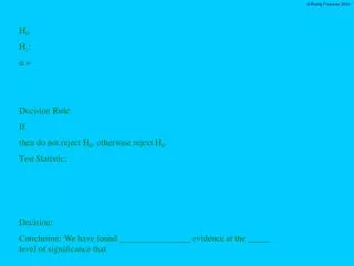
H0: H1: α = Decision Rule: If then do not reject H0, otherwise reject H0. Test Statistic: Decision: Conclusion: We have found ________________ evidence at the _____ level of significance that
H0: H1: α = Decision Rule: If then do not reject H0, otherwise reject H0. Test Statistic: Decision: Conclusion: We have found ________________ evidence at the _____ level of significance that .05 .05
μ1 = μ2 = μ3 not all the means are equal A B C H0: H1: α = Decision Rule: If then do not reject H0, otherwise reject H0. Test Statistic: Decision: Conclusion: We have found ________________ evidence at the _____ level of significance that the means of the number of parts produced per hour using methods: A, B, and C are not all equal. .05 .05
* means coverage is different from text. 2 Groups and > 2 Groups Flowchart 3 4 6 5 7 8 9 10 11 12 13 14 15 paired-difference t-test pp. 315-322 Spearman Rank Correlation test pp. 625-630 yes 1 yes yes Normal populations ? Wilcoxon Signed-Ranks *pp. 614-616 chi-square goodness-of-fit test pp. for the Multinomial Experiment 362-368 and the Normal Distribution 374-376 at least interval level data ? no no 2 Sign Test *pp. 631-634. mean or median yes Z for means with σ1 & σ2 pp. 307-315 yes n1> 30 and n2> 30 ? Related Samples ? yes Normal populations ? Jaggia and Kelly (1stedition) no no Wilcoxon Rank Sum *pp. 616-621 no no σ1 and σ2 both known ? n1> 30 and n2> 30 ? no yes pooled-variances t-test pp. 307-315 yes Normal populations ? no yes σ1 = σ2 ? no unequal-variances t-test p. 307-315 proportion 2 Z for proportions pp. 322-328 Parameter ? variance or standard deviation yes # of groups ? F = S12/S22 pp. 344-354 Normal populations ? no Levine-Brown-Forsythe mean or median yes 1-way ANOVA pp. 386-395 ANOVA OK ? no Kruskal-Wallis *pp. 621-625 more than 2 chi-square df = (R-1)(C-1) pp. 368-374 yes Can we make all fe> 5 ? proportion Parameter ? no Resample and try again. variance or standard deviation yes Hartley’s Fmax *(not in text) Normal populations ? no Default case Levine-Brown-Forsythe
ANOVA OK ? There are three major assumptions for doing an Analysis of Variance (ANOVA) Test: 1. Normality: All the populations are normal. 2. Equality of Variances: The variances of all the populations are equal. 3. Independence of Error: The deviation of each value from the mean of the group containing that value should be independent of any other such deviation.
For this part of the course you may assume the third one (Independence of Error). Care taken when obtaining the sample results should minimize the possibility of a violation of this assumption. However, when data is collected over a lengthy interval of time, this assumption should be checked. We will discuss this further when we get into regression analysis. You are expected to check the other two assumptions: 1. Normality 2. Equality of Variances
This problem has the normality assumption as a given. Later on in the course, we will cover a procedure to test a population to see if it is normally distributed. How do we determine if all the population variances are equal ?
H0: H1: not all variances are equal We can use the following hypothesis test:
If we do not reject the null hypothesis we can perform an ANOVA test to compare the means, but if we do reject the null hypothesis, the ANOVA test is NOT appropriate. If you have one or more of your populations that are definitely NOT normal the ANOVA test is NOT appropriate.
H0: H1: not all variances are equal The flowchart can be used to determine the test statistic needed to test:
* means coverage is different from text. 2 Groups and > 2 Groups Flowchart 3 4 6 5 7 8 9 10 11 12 13 14 15 paired-difference t-test pp. 315-322 Spearman Rank Correlation test pp. 625-630 yes 1 yes yes Normal populations ? Wilcoxon Signed-Ranks *pp. 614-616 chi-square goodness-of-fit test pp. for the Multinomial Experiment 362-368 and the Normal Distribution 374-376 at least interval level data ? no no 2 Sign Test *pp. 631-634. mean or median yes Z for means with σ1 & σ2 pp. 307-315 yes n1> 30 and n2> 30 ? Related Samples ? yes Normal populations ? Jaggia and Kelly (1stedition) no no Wilcoxon Rank Sum *pp. 616-621 no no σ1 and σ2 both known ? n1> 30 and n2> 30 ? no yes pooled-variances t-test pp. 307-315 yes Normal populations ? no yes σ1 = σ2 ? no unequal-variances t-test p. 307-315 proportion 2 Z for proportions pp. 322-328 Parameter ? variance or standard deviation yes # of groups ? F = S12/S22 pp. 344-354 Normal populations ? no Levine-Brown-Forsythe mean or median yes 1-way ANOVA pp. 386-395 ANOVA OK ? no Kruskal-Wallis *pp. 621-625 more than 2 chi-square df = (R-1)(C-1) pp. 368-374 yes Can we make all fe> 5 ? proportion Parameter ? no Resample and try again. variance or standard deviation yes Hartley’s Fmax *(not in text) Normal populations ? no Default case Levine-Brown-Forsythe
A B C H0: H1: not all the variances are equal α = Decision Rule: If then do not reject H0, otherwise reject H0. Test Statistic: Decision: Conclusion: We have found ________________ evidence at the _____ level of significance that that the variances of the number of parts produced per hour using methods: A, B, and C are not all equal. .05 .05
More than 2 groups is an upper-tail test. A B C H0: H1: not all the variances are equal α = Decision Rule: If then do not reject H0, otherwise reject H0. Test Statistic: Decision: Conclusion: We have found ________________ evidence at the _____ level of significance that that the variances of the number of parts produced per hour using methods: A, B, and C are not all equal. .05 .05
More than 2 groups is an upper-tail test. A B C H0: H1: not all the variances are equal α = Decision Rule: If then do not reject H0, otherwise reject H0. Test Statistic: Decision: Conclusion: We have found ________________ evidence at the _____ level of significance that that the variances of the number of parts produced per hour using methods: A, B, and C are not all equal. c = number of groups = 3 .05 Fmax = 5.34 .05
More than 2 groups is an upper-tail test. A B C H0: H1: not all the variances are equal α = Decision Rule: If Fmaxcomputed < 5.34 then do not reject H0, otherwise reject H0. Test Statistic: Decision: Conclusion: We have found ________________ evidence at the _____ level of significance that that the variances of the number of parts produced per hour using methods: A, B, and C are not all equal. c = number of groups = 3 .05 Fmax = 5.34 .05
Calculation of Variations(and Variances) Method MethodMethod A B C n 10 10 10 X = 900 840 810 X2 = 81,882 72,076 67,048
Calculation of Variations(and Variances) Method Method Method A B C n 10 10 10 X = 900 840 810 X2 = 81,882 72,076 67,048
Calculation of Variations(and Variances) Method Method Method A B C n 10 10 10 X = 900 840 810 X2 = 81,882 72,076 67,048 Method A:
Calculation of Variations(and Variances) Method Method Method A B C n 10 10 10 X = 900 840 810 X2 = 81,882 72,076 67,048 Method B:
Calculation of Variations(and Variances) Method Method Method A B C n 10 10 10 X = 900 840 810 X2 = 81,882 72,076 67,048 Method C:
Calculation of Variations(and Variances) Method Method Method A B C n 10 10 10 X = 900 840 810 X2 = 81,882 72,076 67,048 SS = 882 1,516 1,438 S2= 882/9 1,516/9 1,438/9 Smallest variance Largest variance
More than 2 groups is an upper-tail test. A B C H0: H1: not all the variances are equal α = Decision Rule: If Fmaxcomputed < 5.34 then do not reject H0, otherwise reject H0. Test Statistic: Decision: Conclusion: We have found ________________ evidence at the _____ level of significance that that the variances of the number of parts produced per hour using methods: A, B, and C are not all equal. c = number of groups = 3 .05 DonotrejectH0 Fmax = 5.34 Do not reject H0. .05 insufficient
We have found no evidence of any difference in the variances so the ANOVA test is appropriate to use to test the means. We now resume our interrupted hypothesis test of the means.
μ1 = μ2 = μ3 not all the means are equal More than 2 groups is an upper-tail test. A B C H0: H1: α = Decision Rule: If then do not reject H0, otherwise reject H0. Test Statistic: Decision: Conclusion: We have found ________________ evidence at the _____ level of significance that the means of the number of parts produced per hour using methods: A, B, and C are not all equal. .05 where k = # of groups and nT = n1 + n2 + … + nk .05
μ1 = μ2 = μ3 not all the means are equal More than 2 groups is an upper-tail test. A B C H0: H1: α = Decision Rule: If then do not reject H0, otherwise reject H0. Test Statistic: Decision: Conclusion: We have found ________________ evidence at the _____ level of significance that the means of the number of parts produced per hour using methods: A, B, and C are not all equal. dfn = k - 1 = 3 - 1 = 2 dfd = nT - k = 30 - 3 = 27 .05 F = 3.354 where k = # of groups and nT = n1 + n2 + … + nk .05
μ1 = μ2 = μ3 not all the means are equal More than 2 groups is an upper-tail test. A B C H0: H1: α = Decision Rule: If Fcomputed < 3.354 then do not reject H0, otherwise reject H0. Test Statistic: Decision: Conclusion: We have found ________________ evidence at the _____ level of significance that the means of the number of parts produced per hour using methods: A, B, and C are not all equal. dfn = k - 1 = 3 - 1 = 2 dfd = nT - k = 30 - 3 = 27 .05 F = 3.354 where k = # of groups and nT = n1 + n2 + … + nk .05
Calculation of the ANOVA test statistic: The Denominator Variance The denominator is the variance within the groups, but remember variance = variation/df. Therefore, (SW)2 = SSW/dfW. SSW is the variation WITHIN the groups = variation WITHIN group 1 + variation WITHIN group 2 + … + variation WITHIN group k = SS1 + SS2 + … + SSk. Here k = 3, so SSW = SS1 + SS2 + SS3 = 882 + 1516 + 1438 = 3836. dfW = df WITHIN group 1 + df WITHIN group 2 + … + df WITHIN group k = (n1 - 1) + (n2 - 1) + (n3 - 1) = (nT - k) = 27.
Calculation of the ANOVA test statistic: The Numerator Variance The numerator is the variance between the groups, but remember variance = variation/df. Therefore, (SB)2 = SSB/dfB. THE CONCEPT Here the group is the ‘entity.’ If you have k groups then you have (k-1) degrees of freedom, so dfB = (k-1). Recall that the variation of a sample is defined as: SS =å(X-X)2. We will expand this concept to groups. The X represents the group, so we will replace X with a value to represent the group, the mean of the group, X. In the sample variation the X represents the mean of all the X values, so we will replace it with the mean of all values in all the groups, X. The catch is that you must remember to multiply each square by the sample size of the group to account all the values of each group appropriately.
Calculating SSB by Definition The definition formula for SSB is given by: The means of each group are: SSB = 10(90-85)2 + 10(84-85)2 + 10(81-85)2 = 420 The next slide shows an alternative way to calculate SSB.
Alternative Way to Calculate SSB SSB + SSW = SST, the total variation. Therefore, SSB = SST – SSW = SST – 3,836. To calculate SST, just add a column with the totals. Method MethodMethod A B C Total n 10 10 10 30 X = 900 840 810 2,550 X2 = 81,882 72,076 67,048 221,006 Total: Hence, SSB = SST – SSW = 4,256 – 3,836 = 420. With SSB, SSW, and the dfs, the test statistic may be computed.
μ1 = μ2 = μ3 not all the means are equal More than 2 groups is an upper-tail test. A B C H0: H1: α = Decision Rule: If Fcomputed < 3.354 then do not reject H0, otherwise reject H0. Test Statistic: Decision: Conclusion: We have found ________________ evidence at the _____ level of significance that the means of the number of parts produced per hour using methods: A, B, and C are not all equal. dfn = k - 1 = 3 - 1 = 2 dfd = nT - k = 30 - 3 = 27 .05 DonotrejectH0 F = 3.354 Do not reject H0. insufficient .05