Download

1 / 64
690 likes | 1.97k Vues
Differential Amplifiers (Chapter 8 in Horenstein). Differential amplifiers are pervasive in analog electronics Low frequency amplifiers High frequency amplifiers Operational amplifiers – the first stage is a differential amplifier Analog modulators Logic gates Advantages

E N D
Differential Amplifiers (Chapter 8 in Horenstein) • Differential amplifiers are pervasive in analog electronics • Low frequency amplifiers • High frequency amplifiers • Operational amplifiers – the first stage is a differential amplifier • Analog modulators • Logic gates • Advantages • Large input resistance • High gain • Differential input • Good bias stability • Excellent device parameter tracking in IC implementation • Examples • Bipolar 741 op-amp (mature, well-practiced, cheap) • CMOS or BiCMOS op-amp designs (more recent, popular) R. W. Knepper SC412, slide 8-1
Amplifier With Bias Stabilizing Neg Feedback Resistor • Single transistor common-emitter or common-source amplifiers often use a bias stabilizing resistor in the common node leg (to ground) as shown below • Such a resistor provides negative feedback to stabilize dc bias • But, the negative feedback also reduces gain accordingly • We can shunt the common node bias resistor with a capacitor to reduce the negative impact on gain • Has no effect on gain reduction at low frequencies, however • Large bypass capacitors are difficult to implement in IC design due to large area • Conclusion: try to avoid using feedback resistor R2 in biasing network R. W. Knepper SC412, slide 8-2
Differential Amplifier Topology • In contrast to the single device common-emitter (common-source) amplifier with negative feedback bias resistor of the previous slide, the differential ckt shown at left provides a better bypass scheme. • Device 2 provides bypass for active device 1 • Bias provided by dc current source • Device 2 can also be used for input, allowing a differential input • Load devices might be resistors or they might be current sources (current mirrors) • The basic differential amplifier topology can be used for bipolar diff amp design or for CMOS diff amp design, or for other active devices, such as JFETs R. W. Knepper SC412, slide 8-3
Differential Amplifier with Two Simultaneous Inputs • The differential amplifier topology shown at the left contains two inputs, two active devices, and two loads, along with a dc current source • We will define the • differential mode of the input vi,dm = v1 – v2 • common mode of the input as vi,cm= ½ (v1+v2) • Using these definitions, the inputs v1 and v2 can be written as linear combinations of the differential and common modes • v1 = vi,cm + ½ vi,dm • v2 = vi,cm – ½ vi,dm • These definitions can also be applied to the output voltages • Differential mode vo,dm = vo1 – vo2 • Common mode vo,cm = ½ (vo1 + vo2) • Alternately, these can be written as • vo1 = vo,cm + ½ vo,dm • vo2 = vo,cm – ½ vo,dm R. W. Knepper SC412, slide 8-4
Bipolar Transistor Differential Amplifier • Q1 & Q2 are matched (identical) NPN transistors • Rc is the load resistor • Placed on both sides for symmetry, but could be used to obtain differential outputs • Io is the bias current • Usually built out of NPN transistor and current mirror network • rn is the equivalent Norton output resistance of the current source transistor • Input signal is switching around ground • Vref = 0 for this particular design • Both sides are DC-biased at ground on the base of Q1 and Q2 • vBE is the forward base-emitter voltage across the junctions of the active devices • Since Q1 and Q2 are assumed matched, Io splits evenly to both sides • IC1 = IC2 = Io/2 R. W. Knepper SC412, slide 8-5
NPN Bipolar Transistor Physical Structure Dual-Polysilicon Bipolar Transistor Features: • Two polysilicon layers – • P+ for extrinsic base, N+ for emitter • Self-aligned with emitter window opening • Trench Isolation • Oxide lined, polysilicon filled • Shallow Trench Isolation (STI) • Isolate base/emitter active region from collector reach-thru • N-type Pedestal Implant for high fT device • Self-aligned with emitter opening • Limits base push-out (Kirk Effect) • Highly doped extrinsic base lower Rb • Emitter (arsenic) diffused from N+ poly • SiGe Heterojunction BJT: • Typically 10-15% mole fraction of Ge graded into intrinsic base region (as shown), bandgap is narrowed in base, adding drift component to electron velocity Yaun Taur, Tak Ning Modern VLSI Devicees R. W. Knepper SC412, slide 8-6
Bipolar Transistor Operation (1D Device) BJT operation: • An external voltage (0.75-0.85 V) is applied to forward-bias the emitter-base junction • Electrons are injected from the emitter into the base comprising the majority of the emitter current • Holes are injected from the base into the emitter, as well, but their numbers are much smaller, since ND,e >> NA,b • Since XB << Ln in the base, most of the injected electrons get to the collector without recombining with holes. Any holes that do recombine with electrons in the base are supplied as base current. • Electrons reaching the collector are collected across the base-collector depletion region. • Since most of the injected electrons reach the collector and only a few holes are injected into the emitter, or recombine with electrons in the base, IB << IC, implying that the device has a large current gain. R. W. Knepper SC412, slide 8-7
Shown at left are the effects of different NPN bias conditions on the energy bands and the electron concentrations: (a) No bias (thermal equilibrium) • Fermi levels are flat • Electron concentration is ND in emitter and collector and ni2/NA in the base (b) both junctions reverse biased • Increased E-B & B-C barriers • Increase in depletion regions • Electron density in base = ~0 (c) both junctions forward biased • Reduced barrier heights • Electrons injected into base from both emitter and collector (d) forward-biased emitter, reverse-biased collector • Small E-B/large C-B barriers • Electrons injected from emitter • Electron density = ~ 0 at C-B junction and appears linear in base region (small WB) R. W. Knepper, SC412, slide 8-8
BJT Regions of Operation: Ebers-Moll DC Model • Jim Ebers and John Moll developed a dc model for the bipolar transistor which describes the four regions of operation on the Vbe vs Vbc voltage plot shown at the left • Forward active region: • Emitter-base forward biased, collector-base reverse biased • Normal useful region for BJT • Current Gain = ~ 100 typically • Reverse active region: • Collector-base forward biased, emitter-base reverse biased • Transistor is being operated in the inverse mode • Inverse is usually small ~ 1 or < 1 • Saturation region: • Both E-B and C-B forward biased • Base region is flooded with electrons • Cut-off region: • Both junction reverse biased • No current flow • Both junctions are forward-biased the same amount. • No current flows even though the base is loaded with • charge (electrons). • Saturation condition: both junctions forward • biased. Net electron flow from emitter to collector. R. W. Knepper SC412, slide 8-9
Ebers-Moll BJT DC Model Current Equations • The Ebers-Moll model may be used under all junction bias conditions (i.e., forward-active, inverse, saturation, and cut-off) to estimate the terminal currents. R. W. Knepper SC412, slide 8-10
Bipolar Transistor Collector Characteristics • Shown below is a set of BJT (bipolar junction transistor) collector characteristics • IC versus VCE with IB as the parameter • The curves have several regions of operation • At low VCE both the emitter-base junction and the collector-base junction are forward-biased, resulting in what is called saturation in the bipolar transistor • The base volume is flooded with mobile carriers injected from both E-B and C-B junctions • At higher (normal) VCE only the emitter-base junction is forward-biased, while the collector-base junction is reverse-biased, resulting in the normal active (forward mode) region • The carrier concentration is pinned at zero (i.e. very small) at the collector junction, resulting in a linear (triangular) distribution of charge in the base • Non-zero slope in normal active region is caused by base width narrowing due to increase in VCB reverse bias and corresponding increase in C-B depletion region (Early Effect named after Jim Early) • At even higher VCE the transistor enters the onset of avalanche breakdown at the CB junction The non-zero slope in the forward mode region is modeled, as shown below, with a linear term VCE/VA, where VA is the Early Voltage. R. W. Knepper SC412, slide 8-11
NPN DC Characteristics • Top left figure shows a set of collector characteristics (common emitter) for base current stepped from 0 to 30 uA for a SiGe HBT with emitter area of 0.5 x 2.5 um • Very flat curves indicate Early voltage greater than 70 volts. • Gummel plots showing log Ic and log Ib versus VBE indicate excellent SiGe NPN behavior and extremely low recombination current at low VBE • Beta remains constant at about 200 to VBE = 0.9 volt or higher R. W. Knepper SC412, slide 8-12 Harame, et al., IEEE Trans ED, Vol. 48, No. 11, Nov. 2001
Definitions of fT and fmax • Normally the dominant terms in order of significance are the base storage time b, emitter storage time e, and the depletion charge terms (kT/qIc)(Cje + Cjc) • For IBM SiGe NPN technology the last several terms are usually negligible since Re, Rc, and Rns are small • Cuttoff frequency fT can be defined as a series of time constants including base storage time b, emitter storage time e, collector storage time c, and several RC time constants due to emitter and collector depletion capacitances and collector-to-substrate capacitance R. W. Knepper SC412, slide 8-13 IBM SiGe Design Kit Training: Technology, IBM Microelectronics, Burlington, VT, July 2002
SiGe NPN Bipolar and fT versus Current • Plotted at left are the current gain and fT versus collector current for two different emitter width NPN transistors • Both and fT drop off at high current density due to base push-out (called the Kirk Effect) • When the number of injected electrons exceeds the N type doping of the collector region, the base-collector space charge region pushes all the way to the heavily-doped N+ subcollector. • The use of a self-aligned collector pedestal N implant raises the doping in the intrinsic portion of the collector N epi and prevents base push-out until very high current (<1 mA/um2) • Use of a self-aligned pedestal implant limits the increase in Ccb due to the higher collector doping (which is only in the intrinsic portion of the device) • The two curves in the plots are shifted by the area of the emitter. • Using minimum width for the emitter improves base resistance and therefore improves device performance. R. W. Knepper SC412, slide 8-14 Harame, et al., IEEE Trans ED, Vol. 48, No. 11, Nov. 2001
Bipolar Transistor Large-Signal & Small-Signal Models • Shown at the left is a simplified dc large-signal BJT model for normal forward-mode only • The base-emitter junction is modeled as a diode with base current IB as an exponential function of base-emitter bias VBE • The collector current IC is given simply as F times IB • The emitter current IE is given by IC + IB • A small-signal ac bipolar model is shown at the left: • The base-emitter junction is modeled as a parallel RC combination Cbe (stored charge in the base + B-E junction capacitance) with r (= kT/qIB = o/gm) • The collector current is determined by the transconductance term gmVbe in parallel with the output resistance ro • The base resistance is modeled as rb • Collector-to-base and collector-to-substrate capacitances are shown • A simplified expression for fT (shown) can be derived by setting ac current gain to unity R. W. Knepper SC412, slide 8-15
BJT SPICE Model Parameters • Typical SPICE circuit model parameters for a vintage 1 um silicon bipolar technology are given below (from Johns and Martin, Analog Integrated Circuit Design, 1997, p. 65) • The fT would be about 13 GHz, based on the forward base transit time Fof 12 ps • Reverse current gain-bandwidth product would be about 40 MHz based on R of 4 ns • Rb of 500 ohms and Ccb of 18 fF suggest a relatively low fmax of about 7-8 GHz fmax = [fT / 8RbCcb]½ R. W. Knepper SC412, slide 8-16
Small-Signal Model Analysis for Single Input Diff Amp • Consider transistor Q2 with grounded base • dc small-signal model shown in top-left figure • Use the test voltage approach to calculate Q2’s input impedance looking into emitter • Using KCL equations, we can write itest = vtest/r – oib2 where ib2 = - vtest/r • Rearranging and solving for vtest/itest, we have rth2 = vtest/itest = r/(o + 1) = ~ r/o = 1/gm2 • Generally gm2 is large, causing rth2 to act like an ac short • Consider transistor Q1 with Q2 replaced by rth2 • Since rth2 is much smaller than rn (output impedance of Io), we will neglect rn • Writing KCL, we have vin = ib1r1 + ib1(o + 1) rth2 = ib12 r1 • where we assumed r1= r2 • We can now find vout as a function of vin vout = - ic1Rc = - oibRc = - ovinRc/2r1= - ½ gmRcvin • where we have used gm = o/r1 • Small signal gain Av = vout/vin = - ½ gmRc R. W. Knepper, SC412, slide 8-17
Bipolar Diff Amp with Differential Inputs • At left is a bipolar differential amplifier schematic having two inputs that are differential in nature, i.e. equal in magnitude but opposite in phase • The differential input v1 – v2 = va(t) – (-va(t)) = 2va(t) • The common mode input = [va + (-va)]/2 = 0 • A small-signal model for the diff amp is shown below, where the Tx output collector resistance ro is assumed to be >> RC (in parallel) and is neglected • We can derive the small-signal gain due to the differential input by applying KVL to loop A va(t) – (-va(t)) = 2va(t) = ib1r1 – ib2r2 = 2ib1r • since ib1 = -ib2 and r1= r2 • Or, ib1 = va(t)/r and ib2 = - va(t)/r R. W. Knepper SC412, slide 8-18
Bipolar Diff Amp with Differential Inputs (continued) • Solving for the output voltages we can obtain • vo1 = -ic1RC = - oib1RC = - (o/r)va(t)RC and v02 = + (o/r)va(t)RC • We can now find the gain with differential-mode input and single-ended output or with differential-mode input and differential output Adm-se1 = v01/vidm = -gmRC/2 and Adm-se2 = + gmRC/2 Adm-diff = (v01 – v02 )/ vidm = - gmRC • Since corresponding currents on the left and right side of the differential small-signal model are always equal and opposite, implying that no current ever flows throw rn • Node E acts as a “virtual ground” • If the output resistances of Q1 and Q2 are low enough to require keeping them in the analysis, we simply replace RC with the parallel combination of RC||ro for transistor Q1 and Q2 R. W. Knepper SC412, slide 8-19
Small-Signal Model of BJT Diff Amp with CM Inputs • The figure below is the small-signal model for the diff amp with common-mode inputs • v1 = v2 = vb(t) and vicm = ½ (v1 + v2) = vb(t) • The common-mode currents from both inputs flow through rn as shown by the two loops • in = 2(o + 1) ib1 = 2 (o + 1) ib2 • and therefore, vb = ibr + 2(o+ 1)ibrn or ib = vb/[r + 2(o+ 1)rn] • The collector voltages can be found as • v01 = v02 = - oRCvb/[r + 2(o+ 1)rn] = ~ - gmRCvb/ [1 + 2gmrn] • The common-mode gain with single-ended output is given by • Acm-se1 = Acm-se2 = vo1/vicm = vo2/vicm = - gmRC/[1 + 2gmrn] = ~ -RC/2rn • The common-mode gain with differential output is Acm-diff = (vo1 – vo2)/vicm = 0 • Do Example 8.1, p. 488 R. W. Knepper SC412, slide 8-20
BJT Diff Amp Circuit with Both Diff & CM Inputs • The example below illustrates the principle of superposition in dealing with both differential mode and common mode inputs to a diff amp • v1 = vx cos 1t + vy sin 2t and v2 = vx cos 1t – vy sin 2t • Using the definitions of differential mode and common mode inputs, respectively, vidm = v1 – v2 = 2vy sin 2t and vicm = (v1 + v2)/2 = vx cos 1t , • we can obtain vo1 = Adm-se1 vidm + Acm-se1 vicm = - oRC [(vy/ r) sin 2t + (vx/{r + 2 (o+ 1) rn}) cos 1t] • The expression for v02 is similar except that the first term (differential mode) has a minus sign • Note that the common mode output is reduced by the factor (o+ 1) in the denominator R. W. Knepper SC412, slide 8-21
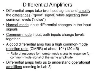
Common-Mode Rejection Ratio • In a differential amplifier we typically want to amplify the differential input while, at the same time, rejecting the common-mode input signal • A figure of merit Common Mode Rejection Ratio is defined as CMRR = |Adm|/|Acm| • where Adm is the differential mode gain and Acm is the common mode gain • For a bipolar diff amp with differential output, the CMRR is found to be CMRR = |Adm-diff|/|Acm-diff| = |- gmRC| / 0 = infinity • In the case of the bipolar diff amp with single-ended output, CMRR is given by CMRR = |Adm-se|/|Acm-se| = | ½gmRC| / | oRC/[r + 2(o+ 1)rn]| = [r + 2(o+ 1)rn]/2r = ~ orn/r = gmrn = ICrn/VT = Iorn/2VT • since o = gmr and VT is defined as kT/q • CMRR is often expressed in decibels, in which case the definition becomes • CMRR = 20 log (|Adm|/|Acm|) R. W. Knepper SC412, slide 8-22
BJT Diff Amp Input and Output Resistance Input Resistance: • For differential-mode inputs, the input resistance can be found as • rin-dm = (v1 – v2)/ib1 = (va – (-va)) / (va/r) = 2var/va = 2r • For common-mode inputs, the input resistance is quite different • rin-cm = ½(v1 + v2)/ib1 = vb / [vb /(r+ 2(o+ 1)rn)] = r + 2(o+ 1)rn Output Resistance: • For differential outputs, we can use the test voltage method (below) for deriving the output resistance where all inputs are set to zero • Since ib1 and ib2 are both zero, we have itest = vtest/(RC + RC) = vtest/2RC or rout-diff = 2RC • For single-ended outputs, rout-se = RC || ro = ~ RC R. W. Knepper SC412, slide 8-23
Bipolar Diff Amp Biasing Considerations • A bipolar differential amplifier with ideal current source and resistor loads is shown • It is assumed that components are matched sufficiently such that bias current Io is split evenly between the left and right-hand legs • Node E will take a voltage value such that IC1 = IC2 = Io/2 when v1 = v2 = 0 • By using the Ebers-Moll dc model for the NPN transistors, we can determine the voltage at node E IE = IEO [exp (qVBE/kT) – 1] = IEO exp (qVBE/kT) = Io/2 or, VBE = (kT/q) ln (IE/IEO) • Typically, VBE = 0.75-0.85 V in modern NPN transistors • It is important to design RC such that vout never drops so low so as to force Q1 or Q2 into saturation. R. W. Knepper SC412, slide 8-24
BJT Diff Amp with Simple Resistor Current Source • The simplest approach to building a current source is with a resistor • Given that node E is one VBE drop below GND, we can choose RE to provide the desired bias current Io • RE = (0 – VBE – VEE) / Io • Preventing saturation in Q1 and Q2 provides an upper bound for RC • RC ~ < (VCC – 0)/(Io/2) = 2 VCC / Io • Look at Example 8.3 in text. • Do problem 8.31 in class. R. W. Knepper SC412, slide 8-25
Example 8.3: Diff Amp with Complete Bias Design • Design Conditions • Differential-mode, single-ended gain > = 50 • Common-mode, single-ended gain < = 0.2 • Completed design is shown above • In class Exercise: 8.4, 8.5, & 8.6 R. W. Knepper SC412, slide 8-26
BJT Diff Amp with BJT Current Source • The expression for common-mode gain on slide 8-20 (-RC/2rn) shows that in order to reduce Acm, we want to make the effective impedance of the current source very high • Using a resistor to generate the current source limits our design options in making rn (RE in this case) high • An alternate method of generating Io is to use an NPN transistor current source similar to that shown at the left • Q3 is an NPN biased in the forward active region so that rn (given by the inverse slope of the collector characteristics) is very high • RA and RB form a voltage divider establishing VB = VEE x RA/(RA + RB) where VEE is <0 • The voltage across RE can be used to find Io • VRE = VB – Vf – VEE • Io = (VB – Vf – VEE)/RE is the bias current provided to the diff amp R. W. Knepper SC412, slide 8-27
Small Signal Model of BJT Current Source Transistor • Find the small-signal resistance looking into the collector of Q3 on slide 8-27 diff amp • If RE were = 0, then the solution becomes simply ro, since the incremental base current ib3 would, in fact, be 0 • With a finite feedback resistor RE, we need to use KVL and KCL to derive an expression for rn (See Example 8.4 in text) • Apply a test current itest and find vtest • Obtain v3 by applying KVL to the 3 left-most resistors to obtain ib3 and multiply by r3 v3 = -itest RE r3 /[RE + r3 + RP] • If we multiply this result by gm3 and substract from itest, we obtain io3 which can be used to find vo3 by multiplying by r03 vo3 = itest{1 + gm3RE r3 /[RE + r3 + RP]}ro3 • ve can be found as (itest + ib3) x RE ve = itest (r3 + RP) RE/(RE + r3 + RP) • Adding vo3+ ve = vtest, we obtain rn = vtest/itest rn = RE || (r3 + RP) + r03 [1 + oRE/(RE+ r3+RP)] Do Exercise 8.8 and 8.9 in class. R. W. Knepper SC412, slide 8-28
Bipolar Current Mirror Circuit • A method used pervasively in analog IC design to generate a current source is the current mirror circuit • In the bipolar design arena, the method is as follows: • A reference current is forced through an NPN transistor connected as a base-emitter diode (base shorted to collector), thus setting up a VBE in the reference transistor • This VBE voltage is then applied to one or more other “identical” NPN transistors which sets up the same current Iref in each one of the bias transistors • As long as the bias transistor(s) is (are) identical to the reference transistor, and as long as the bias transistor(s) is maintained in its normal active region (where collector current is independent of the collector-emitter voltage), then the current in the bias transistor(s) will be identical to the current in the reference transistor. • Variations on the basic current mirror circuit can be used to generate 2X or 3X or maybe 10X the original reference current by using several bias NPN transistors in parallel • Or alternately, by using an emitter that has 2X or 3X or 10X emitter stripes and is otherwise identical to the reference transistor • Advantages • One reference current generator can be used to provide bias to several stages • Very high incremental output impedance can be obtained from the current mirror • The technique can be used in both bipolar and in CMOS/BiCMOS technologies R. W. Knepper SC412, slide 8-29
Bipolar Current Mirror Bias Circuit Design • Design procedure: • Given RA and the IC vs VBE characteristics of the NPN reference device, we can determine IA, or • Given the desired IA and the IC vs VBE characteristics of the NPN reference device, we can choose RA • We can find IA by dividing the voltage drop across RA by the resistance value • IA = (VCC – VBE1 – VEE) / RA • Assuming that the two base currents are small, we can say IA = Iref • Because of the current mirror action, the VBE1 set up in Q1 to sustain current Iref will be equal to VBE2, the base-emitter voltage in Q2 • Therefore, Io = Iref = IA • Note: corrections for IB1 and IB2 can easily be made is needed • Note 2: Q2 must be maintained in its forward active region R. W. Knepper SC412, slide 8-30
BJT Diff Amp with Current Mirror Bias (Ex. 8.5) • Design Objectives: • Diff amp with 1.5 mA in each leg • 5V drop across load resistors • VCC = +10V, VEE = -10V • Design Procedure: • Set Io = IA = 3 mA • RA = (0 – VBE = VEE)/3mA = 3.1K • where we used VBE = 0.7 volt • RC1 & RC2 can be found as follows: • RC1 = RC2 = 5V/1.5 mA = 3.3K • Check VCE of Q2, Q3, and Q4 to see if they are in normal active region • VC = VCC – 1.5 mA x 3.3K = 5V • VE = 0 – VBE = -0.7V • VCE = 5 – (-0.7) = 5.7V for Q2 and Q3 • For Q2 VCE = -0.7V – (-10) = -9.3V • Calculate power in each device • PQ3 = PQ4 = 1.5mA x 5.7V = 8.6 mW • PQ2 = 3 mA x 9.3V = 28 mW • PQ1 = 3 mA x 0.7V = 2.1 mW R. W. Knepper SC412, slide 8-31
BJT Current Mirror Feeding 2-stage Diff Amp • The example below shows a 2-stage bipolar diff amp fed from two current sources with a single current mirror • Reference current 0.93mA is determined by placing (0 – VBE – VEE) across a 10K bias resistor • The reference current is used for the first differential stage with 0.47 mA on each leg • The second differential stage is to have double the bias current of the first stage • This is accomplished by using two bias NPN transistors in parallel giving 1.86 mA bias current with 0.93 mA flowing on each leg (Q7 and Q8) • Check the VCE of each device to check for normal active region and calculate power in circuit. • The total circuit power is found by computing the sum of the three current source currents multiplied by the source-sink voltage differential for each. • Q1: 0.93mA x 10V = 9.3mW • Q2: 0.93mA x 20V = 18.6mW • Q3/Q4: 1.86mA x 20V = 37.2 mW • Total circuit power = 65.1 mW R. W. Knepper SC412, slide 8-32
Bipolar Widlar Current Source • A special use of the current mirror is the Widlar Current Source (shown at left) • A resistor in the emitter of Q2 is used to reduce the current Io in Q2 to a value less than that in Q1 • Io can be set to a very small value by increasing the R2 value • Design procedure: • As in the standard current mirror, we can find Iref as follows: Iref = (VCC – VEE – VBE1)/RA • But, in contrast to the standard current mirror, VBE2 will not be equal to VBE1 VBE1 = VBE2 + IE2R2 • Using the Ebers-Moll model for emitter current IE = IEO (exp[VBE/VT] – 1) = ~ IEO exp[VBE/VT] • We can invert this expression and insert it into the above equation for VBE1 to obtain IE2 = (VT/R2) ln(IE1/IE2) = Io = (VT/R2) ln(Iref/Io) • Since this is not a closed form solution, an iterative approach can be used to solve for Io by starting with a best guess. • Example iteration procedure: • Assume that Iref = 1 mA and R2 = 500 ohms. Guess Io inside ln term. Find LHS Io. • Initial guess = 0.5 mA, then Io = 0.036mA • Try a guess of 0.2 mA, then Io = 0.083mA • Try a guess of 0.1mA, then Io = 0.119mA • Try a guess of 0.11mA, then Io = 0.114mA Close enough!! R. W. Knepper SC412, slide 8-33
Small-Signal Model for Widlar Current Source Q1 • The incremental output impedance (looking into Q2 collector) of Widlar Current Source is similar to the expression derived for the BJT current source (slide 8-28) except that RP must be replaced by the incremental resistance at the base of Q1 • From the model below, the incremental resistance at the base of Q1 is given by r1 || 1/gm1 || ro1 || RA = ~ [r1/(o1 + 1)] || RA • Thus, the output impedance seen looking into the collector of the Widlar Current Source is given by rn = R2 || (r2 + RP) + r02 [1 + o2R2/(R2+ r2+RP)] • where the above expression is to be used in place of RP • However, with a number of approximations and using the relation IoR2/VT= ln (Iref/Io), the expression may usually be simplified to rn = r02 [1 + ln (Iref/Io)] • Look over Example 8.9 in text. R. W. Knepper SC412, slide 8-34
NMOS Differential Amplifier Circuit • Shown below is a differential amplifier circuit built with NMOS technology • Q1 and Q2 comprise the diff amp active gain transistors • fed by a current mirror Q7 and Q5 • Q3 and Q4 are NMOS enhancement mode saturated loads • Q6 and Qref are used for biasing the NMOS current mirror • Current Io is presumed to split equally on the left and right legs of the diff amp • The voltage rails are now called VDD and VSS • Before going into the biasing and small signal models, we will take a look at MOSFET devices and models R. W. Knepper SC412, slide 8-35
MOSFET Transistor DC Current Modes • DC Current Modes: • Cut-off: Vgs VT • Ids = 0 (interface is depleted) • Linear Region: Vgs > VT, Vgs – VT > Vds • Ids = N Vds (Vgs – VT – Vds/2) • interface is inverted and not pinched off at drain (Fig. a) • Pinch-off Point: Vgs > VT, Vds = Vdsat • channel pinches off at the drain junction • simple theory: Vdsat = Vgs – VT (Fig. b) • Saturated Region: Vgs > VT, Vgs – VT < Vds • Ids = ½N (Vgs – VT)2 • interface is inverted and pinched off at drain • further increase in Vds occurs across pinch-off depletion region (Fig. c) • N = NCox (W/L)N where N is the mobility of electrons in the channel, Cox is the gate capacitance per unit area, W is the device width and L is the device effective channel length R. W. Knepper SC412, page 8-36
MOSFET DC Characteristics: linear vs saturation • If the linear Ids expression from the previous chart is plotted with increasing Vds, one observes a maximum at Vds = Vgs – Vt after the current reduces in a parabolic fashion. • In fact, the charge in the channel Qn(y) goes to zero at Vds = Vgs – Vt • The voltage Vds = Vgs – Vt = Vdssat is the pinch-off voltage where the channel pinches off at the drain junction. • Further increase in Vds simply increases the voltage between the drain and the channel pinch-off point, and does not increase the voltage V(y) along the channel. • Therefore, IDS remains constant for further increases in Vds and we say the device is in the saturation region (or active region) with IDS = ½ n Cox (W/L) (Vgs – Vt)2 • The transconductance in saturation • can be found by differentiating the • expression for IDS with Vgs, giving • gm = nCox (W/L) (Vgs – Vt) • = [2 nCox (W/L) IDS]½ R. W. Knepper SC412, slide 8-37
IDS versus VDS for A Real Device Channel length modulation: • As VDS increases, in fact, there is some non-zero slope on the IDS vs VDS characteristic • The increase in IDS with VDS is caused by a shortening of the effective channel length Leff with increasing VDS due to an increase in the depletion region thickness from the channel tip to the drain junction • Substituting for L, from the expression for the thickness of an abrupt junction (with a square root dependence on reverse biased voltage), one can obtain a modified expression for the current IDS in saturation (active region) as shown below. • From this new expression one can derive an expression for the output drain-source resistance of the NMOS transistor in the saturation region as • rds = 1/(dIDS/dVDS) = 1/(IDS) • where is defined below and kds = [2SIo/qNA]½ R. W. Knepper SC412, slide 8-38
MOSFET Capacitance Model • The MOSFET capacitances (gate-to-source, gate-to-drain, gate-to-substrate, source-to-substrate, and drain-to-substrate) are illustrated in the drawing at left and summarized in the table below • Cov is an overlap capacitance due primarily to lateral diffusion of the source and drain junctions, but also includes fringing capacitance Cov =~ 2/3 Cox W xj • where xj is the junction depth • The gate-to-channel capacitance is evenly divided between source and drain in the linear (triode) region, but is effectively connected only to the source at pinchoff • Integration of the channel charge shows that only 2/3 of Cgc becomes part of Cgs in the saturation (active) region • A similar reasoning is used to partition Ccx (CCB in picture) between Csx and Cdx • Cgx (gate-to-substrate) is zero when Vgs > Vt, but increases to CoxW(L - 2L) in the accumulation region. R. W. Knepper SC412, slide 8-39
MOSFET High Frequency Figures of Merit Unity gain bandwidth product fT (frequency where current gain falls to 1): • Assume that a small signal sinusoidal source vGS = Vpsin(t) is applied to the gate • Input current is given by iG = CG (dvGS/dt) = CG Vpcos(t) = (Cgs + Cgd) Vpcos(t) • Output current is given by iDS = gm vGS from the definition of gm • If we write the magnitude of the ac current gain, we have |iDS/iG| = |gmvGS / (Cgs + Cgd)Vpcos(t)| = gm/(Cgs + Cgd) • Where we have replaced Vpcos(t) with vGS since we are using only the magnitudes • Setting the magnitude of the current gain to unity, we obtain fT = gm/2(Cgs + Cgd) • Because of the manner in which it is derived, fTneglects series gate resistance rg and capacitance on the output, such as Cgd. Unity power gain bandwidth product fmax (frequency where power gain falls to 1): • A useful expression for the unity power gain point fmax is given by fmax = [fT / 8rgCgd]½ • These figure of merits are useful for technology comparisons and are also often used in high frequency amplifier design R. W. Knepper SC412, slide 8-40
Long-Channel versus Short-Channel Considerations • Consider the current gain bandwidth product fT as a function of device parameters: fT = gm / 2Cgs = µnCox(W/L)(Vgs – Vt) / (2/3)WLCox = 1.5µn(Vgs – Vt) / L2 • where we have assumed the gate capacitance is predominantly the Cgs portion • Note that fT increases with small L (inverse with L2) and with increasing Vgs • This is a result based only on a long-channel assumption. • As the channel shortens, the electric field increases beyond the point where mobility is constant any longer (typical of today’s advanced CMOS technology) • Scattering of electrons by optical phonons causes the drift velocity to saturate at about 1E7 cm/sec, occurring at an electric field Esat = ~ 1E4 V/cm. • Beyond this point further increases in E field result in diminishing increases in carrier velocity • This effect represents itself in the IDS current equation by a reduction in Vdssat below Vgs – Vt thus reducing IDSsat to less than ½ µnCox(W/L)(Vgs – Vt)2 • If we redefine Vdsat to be “determined” by the minimum of (Vgs – Vt) and LEsat (i.e. sort of having (Vgs – Vt) and LEsat in parallel), we can write Vdsat = [(Vgs – Vt)(LEsat)] / [(Vgs – Vt) + (LEsat)] • We can then rewrite the current equation as IDS = ½ µnCox(W/L)(Vgs – Vt)(Vdsat) = WCox(Vgs – Vt) vsat [1 + LEsat/(Vgs – Vt)]–1 • where vsat is the saturation velocity given by ½µnEsat and µn is the low field mobility • At short L, the equation becomes IDS = ½ µnCoxW(Vgs – Vt)Esat which is independent of L R. W. Knepper SC412, slide 8-41
Small Signal Model for a MOSFET • The main contribution to the output current is the source gmvgs and is given by the expression below • The current source gsvsx is due to the possibility that the source and substrate (bulk) voltages may not be the same. gs = IDS/VSX = gm / [2(Vsx + |2F|)½] • where = [{2qNA}]/Cox and 2F is the band bending at strong inversion (from Vt equation) • In essence gs is a back-gate transconductance which contributes current due to bulk-charge voltage change • rds accounts for the finite output impedance and is given by rds = 1 / IDS • where is the output impedance constant (defined on slide 8-38) R. W. Knepper SC412, slide 8-42
MOSFET SPICE Model • Level 3 SPICE model parameters are shown in the table at the left. • The following parameters are given in text for a 0.5 um technology: (PMOS in parentheses if different than NMOS) • PHI=0.7, TOX=9.5E-9, XJ=0.2U • TPG=1 (-1), VTO=0.7 (-0.95) • DELTA=0.88(0.25), LD=5E-8 (7E-8) • KP=1.56E-4 (4.8E-5), UO=420 (130) • THETA=0.23 (0.20), RSH=2.0 (2.5) • GAMMA=0.62 (0.52) • NSUB=1.4E17 (1.0E17) • NFS=7.2E11 (6.5E11) • VMAX=1.8E5 (3E5) • ETA=0.02125 (0.025) • KAPPA=0.1 (8) • CGDO=CGSO=3.0E-10 (3.5E-10) • CGBO=4.5E-10, CJ=5.5E-4 (9.5E-4) • MJ=0.6 (0.5), CJSW=3E-10 (2E-10) • MJSW=0.35 (0.25), PB=1.1 (1.0) R. W. Knepper SC412, slide 8-43
MOSFET Transistor at Threshold (N-FET) Kang & Leblebici, CMOS Digital Integrated Circuits, 1999 • MOSFET with Vgs > VT causes formation of a channel (inversion layer) connecting source to drain • With Vds > 0, a positive current Ids flows from drain to source (N-FET) • Depletion layer exists from source, drain, & channel N region to P substrate • At Vgs = VT, bands are bent by |2F| at oxide-silicon interface • Threshold definition (by summation of charges in gate, oxide, channel, and bulk: • VTN = - Qfc/Cox + {2qNA(2F + Vsx)}/Cox + MS + 2F for N-FET’s • VTP = - Qfc/Cox - {2qNA(|2F + Vsw|)}/Cox + MS + |2F| for P-FET’s R. W. Knepper SC412, page 8-44
oxide oxide gate gate N + N N+ P+ P+ source source P substrate drain drain N well N channel device P channel device CMOS NFET and PFET Transistors VTN = - Qfc/Cox + {2qNA(2F + Vsx)}/Cox + MS + 2F for N-FET’s VTP = - Qfc/Cox - {2qNA(|2F + Vsw|)}/Cox + MS + |2F| for P-FET’s • Threshold Voltage is a square root function of source-to-substrate per chart at left. Applies to both N and P devices using |Vsx+2F| • Implications for circuit applications where the source voltage rises significantly above ground potential. R. W. Knepper SC412, page 8-45
DC Bias Considerations for NMOS Diff Amp • It is desired to design the NMOS diff amp (below) with device symmetries in such a way that VDS3 = VDS4 = VDSref • Since Io/2 = Iref/2 flows through Q3 and Q4, and since Qref, Q3, and Q4 are all biased in their saturation (active) regions where IDS = ½ nCox (W/L)(VGS – VT)2 = K(VGS – VT)2 , we can obtain VGS3 = VGS4 = VGSref if W3 = W4 = ½ Wref • This condition will be met independent of other device parameter values as long as their ratios remain fixed, i.e. good tracking between devices exists • Assuming that the W of Q6 and Q7 are identical to that of Qref, then we can see that the above current equation will require that VGS6 = VGS7 = VGSref = 1/3 (VDD – VSS), where we have neglected any dependence of VT on Vsx. If we set the current in Q3 to that in Qref, we can obtain the following expression VDS3 = (VDD – VSS)/3 + [1 - ]VT where = (Kref/2Kpu)½ Thus, setting Kref = 2Kpu leads to VDS3 = 1/3 (VDD – VSS) or Vout1 = VDD – VDS3 = 2/3 VDD + 1/3 VSS R. W. Knepper SC412, slide 8-46
Modified MOSFET Current Mirror Reference Ckt • At left is a modified current mirror reference circuit in which four saturated NMOS transistors split the voltage between VDD and VSS • Assuming that each transistor is designed with the same W/L ratio, the reference device VDS will be ¼ of VDD – VSS • Assuming we design transistor Q3 with ½ the W of Qref (as on the previous chart), then we will have VDS3 = ¼ (VDD – VSS) and Vout1 = (3VDD + VSS)/4 • For n reference devices in series, we can generalize the above to Vout1 = [(n-1)/n]VDD + VSS/n • Exercises 8.15 and 8.16 R. W. Knepper SC412, slide 8-47
Small-Signal Model for the NMOS Diff Amp Ckt • The small signal model below is the starting point for deriving the gain expressions for the NMOS differential amplifier • Each transistor is modeled by the gate transconductance current source, the back-gate transconductance current source, and the incremental ac impedance of the device in saturation • Note the opposite direction of the back-gate (body effect) term is due to the use of bulk-to-source voltage rather than source-to-bulk voltage • The current mirror current source is modeled simply by its output impedance (in saturation) • Each transistor is presumed to be in its saturation (constant current) region R. W. Knepper SC412, slide 8-48
Small-Signal Model for NMOS Diff Amp Load Imp • We can simplify the equivalent circuit of the previous chart by replacing the load transistors by their Thevenin equivalent resistance looking into their source nodes. • Using the test voltage method (shown at left), we can obtain • rth = 1/[gm + gmb + (1/ro)] • = [1/gm(1 + )] || ro • where gmb = gm • and = {(2/qNA)/(Vsx + 2F)}½ • Generally we can assume = 0.2, I.e. the back-gate (body) effect adds about 20% to the gate transconductance (if we define the voltage as bulk-to-source) or reduces the gate transconductance about 20% (using the voltage as source-to-substrate). • With the above approximation for the load device, we can simplify the NMOS diff amp incremental model to that shown on the following slide R. W. Knepper SC412, slide 8-49
Simplified Small-Signal Circuit Model of NMOS Diff Amp • Differential mode gain can be found from the small signal circuit below Adm-se1 = -Adm-se2 = - ½ gm1 [(1/gm3(1 + 3)) || ro3 || ro1] Adm-diff = - gm1[(1/gm3(1 + 3)) || ro3 || ro1] and gm = [2nCox (W/L) IDS]½ • where we have assumed matched pairs Q1 & Q2 and Q3 & Q4 • Resistances r01 and r03 are often large enough to be neglected relative to 1/gm • Common mode gain can also be found from the small signal circuit below Acm-se1 = Acm-se2 = -gm1rth3/[1 + 2ro5gm1(1 + 1)] = ~ rth3/2ro5(1 + 1) • Input impedance is assume to be infinite • Output impedance is given by rout-se = rth3 = 1/gm3(1 + 3) and rout-diff = 2/gm3 (1 + 3) R. W. Knepper SC412, slide 8-50