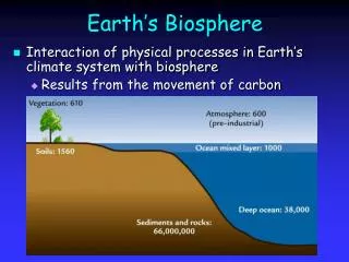
Earth’s Biosphere
Earth’s Biosphere. Interaction of physical processes in Earth’s climate system with biosphere Results from the movement of carbon. Carbon Cycle. Carbon moves freely between reservoirs Flux inversely related to reservoir size. Photosynthesis. Sunlight, nutrients, H 2 O

Earth’s Biosphere
E N D
Presentation Transcript
Earth’s Biosphere • Interaction of physical processes in Earth’s climate system with biosphere • Results from the movement of carbon
Carbon Cycle • Carbon moves freely between reservoirs • Flux inversely related to reservoir size
Photosynthesis • Sunlight, nutrients, H2O • Transpiration in vascular plants • Efficient transfer of H2O(v) to atmosphere • Oxidation of Corg • Burning • Decomposition
Terrestrial Photosynthesis • CO2 and sunlight plentiful • H20 and correct temperature for specific plants not always sufficient • Biomass and biome distribution controlled by rainfall and temperature
Local Influence on Precipitation • Orographic precipitation influences distribution of biomass and biomes • Influences the distribution of precipitation
Marine Photosynthesis • H2O, CO2 and sunlight plentiful • Nutrients low (N, P) • Nutrients extracted from surface water by phytoplankton • Nutrients returned by recycling • Upper ocean (small) • Upwelling (high) • External inputs (rivers, winds)
Ocean Productivity • Related to supply of nutrients • Nutrient supply high in upwelling regions • Equatorial upwelling • Coastal upwelling • Southern Ocean • Wind-driven mixing • Short growing season • Light limitation
Productivity – Climate Link • “Biological Pump” – photosynthesis takes up CO2 and nutrients, plants eaten by zooplankton, dead zooplankton or excreted matter sinks carrying carbon to sediments
Export – Removal of Carbon • For every 1000 carbon atoms taken up by phytoplankton • 50-100 sink below 100 m • 10 are exported to depths below 1 km • Stored for millennia • 1 carbon atom is buried in deep sea sediments • Sequestered for eons
HNLC • Growth in regions limited by micronutrients (Fe) • High nutrient low chlorophyll (N. Pacific, SO) • Higher production linked with removal of CO2
Effect of Biosphere on Climate • Changes in greenhouse gases (CO2, CH4) • Slow transfer of CO2 from rock reservoir • Does not directly involve biosphere • 10-100’s millions of years • CO2 exchange between shallow and deep ocean • 10,000-100,000 year • Rapid exchange between ocean, vegetation and atmosphere • Hundreds to few thousand years
Increases in Greenhouse Gases • CO2 increase anthropogenic and seasonal • Anthropogenic – burning fossil fuels and deforestation • Seasonal – uptake of CO2 in N. hemisphere terrestrial vegetation • Methane increase anthropogenic • Rice patties, cows, swamps, termites, biomass burning, fossil fuels, domestic sewage
Climate Archives • Four major archives of climate records • Sediments • Ice • Corals • Trees • Each archive has different time span, resolution and ease of dating
Understanding Climate Change • Understanding present climate and predicting future climate change requires • Theory • Empirical observations • Study of climate change involves construction (or reconstruction) of time series of climate data • How these climate data vary across time provides a measure (quantitative or qualitative) of climate change • Types of climate data include temperature, precipitation (rainfall), wind, humidity, evapotranspiration, pressure and solar irradiance
Contemporary & Past Climate • Contemporary climate studies use empirically observed instrumental data • Temperature records available from central England beginning in the 17th century • Period traditionally associated with instrumental records extends back to middle of the 19th century • Climate change from periods prior to the recording of instrumental data • Must be reconstructed from indirect or proxy sources of information
Climate Construction from Instrumental Data • Contemporary climate change studied by constructing records (daily, monthly and annual) which have been obtained with standard equipment • Temperature • Rainfall • Humidity • Wind
Paleoclimate Reconstructions • Climate varies over different time scales and each periodicity is a manifestation of separate forcing mechanisms • Different components of the climate system change and respond to forcing factors at different rates • To understand the role each component plays in the evolution of climate we must have a record longer than the time it takes for the component to undergo significant change
Paleoclimatology • Study of climate change prior to the period of instrumental measurements • Instrumental records span only a fraction (<10-7) of Earth's climatic history • Provide a inadequate perspective on climatic variation and the evolution of the climate today and in the future • A longer perspective on climate variability can be obtained by the study of natural climate-dependent phenomena • Such phenomena provide a proxy record of the climate
Paleoclimate Proxy Records • Many natural systems are dependent on climate • It may be possible to derive paleoclimatic information from them • By definition, such proxy records of climate all contain a climatic signal • The signal may be weak and embedded in a great deal of (climatic) background noise • Proxy material acts as a filter, transforming climate conditions in the past into a relatively permanent record • Deciphering that record can often be complex
Proxy Data • Proxy material can differ according to • Its spatial coverage • The period to which it pertains • Its ability to resolve events accurately in time • For example • Ocean floor sediments, reveal information about long periods of climatic change and evolution (107 years), with low-frequency resolution (103 years) • Tree rings useful only during the last 10,000 years, but offer high frequency (annual) resolution • The choice of proxy record (as with the choice of instrumental record) depends on physical mechanism under review
Factors to Consider • When using proxy records to reconstruct paleoclimates one must consider • The continuity of the record • The accuracy to which it can be dated • Ocean sediments may be continuous for over 1 million years but are hard to date • Ice cores may be easier to date but can miss layers due to melting and wind erosion • Glacial deposits are highly episodic, providing evidence only of discrete events in the past • Different proxy systems have different levels of inertia with respect to climate • Some systems vary in phase with climate forcing • Some systems lag behind by as much as several centuries
Steps in Reconstructing Climate • Paleoclimate reconstruction proceeds through a number of stages • The 1st stage is proxy data collection, followed by initial analysis and measurement • This results in primary data • The 2nd stage involves calibration of the data with modern climate records • The secondary data provide a record of past climatic variation • The 3rd stage is the statistical analysis of this secondary data • The paleoclimatic record is statistically described and interpreted
Proxy Calibration • The uniformitarian principle is typically assumed • Contemporary climatic variations form a modern analog for paleoclimatic changes • However the possibility always exists that paleo-environmental conditions may not have modern analogs • The calibration may be only qualitative, involving subjective assessment, or it may be highly quantitative
Proxy Calibration: An Example • Emiliania huxleyi is one of 5000 or so species of phytoplankton • Most abundant coccolithophore on a global basis, and is extremely widespread • Occurs in all except the polar oceans • Produces unique compounds • C37-C39 di-, tri- and tetraunsaturated methyl and ethyl ketones
Emiliania huxleyi Blooms • E. huxleyi can occur in massive blooms • 100,000 km2 • During blooms E. huxleyi cell numbers usually outnumber those of all other species combined • Frequently they account for 80 or 90% of the total number of phytoplankton SeaWiFS satellite image of bloom off Newfoundland in the western Atlantic on 21 July 1999
UK’37 Varies with Temperature • Alkenone unsaturation global calibration • UK’37 determined in core top sediment samples • SST from from Levitus ocean atlas • Figure from Muller et al. (1998)