Download
1 / 58
580 likes | 741 Vues
Modelling of transient vegetation and soil related processes. Patrick Samuelsson Swedish Meteorological and Hydrological Institute patrick.samuelsson@smhi.se. The Rossby Centre Regional Climate Model Land Surface Scheme (LSS) (Samuelsson and Gollvik)

E N D
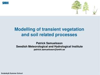
Modelling of transient vegetation and soil related processes Patrick Samuelsson Swedish Meteorological and Hydrological Institute patrick.samuelsson@smhi.se
The Rossby Centre Regional Climate Model Land Surface Scheme (LSS) (Samuelsson and Gollvik) • The ECMWF TESSEL LSS (Viterbo et al.)
Outline • Introduction • Net radiation • Physiography • Surface fluxes • Surface resistances • The forest tile • Interception of rain • Soil heat storage • Soil properties • Soil water • Interception of snow
The role of the land surface inNWP/climate models • Act as a lower boundary for the atmosphere. • Provide diagnostic values of 2m temperature and humidity and 10m wind speed. • Partitioning between sensible heat and latent heat determines soil wetness, acting as one of the forcings of low frequency variability (e.g. extended drought periods). • At higher latitudes, soil water only becomes available for evaporation after the ground melts. The soil thermal balance and the timing of snow melt (snow insulates the ground) also controls the seasonal cycle of evaporation. • The outgoing surface fluxes depend on the albedo, which in turn depends on snow cover, vegetation type and season. Viterbo, 2004
The role of the land surface in NWP/climate models The water balance components Precipitation ERA40:2.2 mm d-1 ERA40:-1.4 mm d-1 Evapotranspiration Storage of water ERA40:-0.9 mm d-1 Runoff ERA40 from P. Viterbo
Definitions of evaporation Unstressed evaporation or Potential evapotranspiration (dry vegetation) Potential evaporation (wet vegetation) Field capacity
The hydrological rosette(Dooge, 1992) B-C: Soil water has decreased to a level where it starts to limit the rate of evaporation. A-B: After a long episode of rainfall soil moisture is available in abundance. The atmosphere controls the rate of evaporation. C-D: Precipitation refills the soil water by infiltration. D-A: Maximum soil water level is reached. All precipitation from this point goes to runoff.
The role of the land surface in NWP/climate models model The energy balance components Incoming shortwave (S↓) ERA40 NetSW:134 Wm-2 EvapotranspirationLatent heat (LE) ERA40:-40 Wm-2 Incoming longwave (L↓) ERA40 NetLW:-65 Wm-2 Sensible heat (H) ERA40:-27 Wm-2 Phasechanges Storage of heat ERA40 from P. Viterbo
Surface net radiation Albedo Emissivity Surface temperature Arya, 1988
Surface net radiationin the forest Rnforc Rnforc The sky view factor divides the radiationbetween the canopy and the forest floor: Rnforsn Rnfors
(1) EF = (Latent heat)/(Net radiation) (2) Bo = (Sensible heat)/(Latent heat) Feedback mechanisms involvingland surface processes • Surface evaporative fraction1 (EF), impacting on low level cloudiness, impacting on surface radiation, impacting on … • Bowen ratio2 (Bo), impacting on cloud base, impacting on intensity of convection, impacting on soil water, impacting on … P. Viterbo (2004)
History of land-surface modelling (Viterbo, 2002) • Richardsson (1922): In his book on numerical weather prediction he identified all the principles used by most current LSS. • Manabe (1969): The “bucket model” for evaporation and runoff. • Deardorff (1978) introduced the importance of vegetation in controlling the evaporation. Many of today’s LSS are build on these principles. • Jarvis (1976) described how different stress functions affect the stomatal conductance.
The mixture contra the tile approach (Koster and Suarez, 1992) The Mixture approach The Tile approach Coniferous forest Most schemessomewhere inbetween Averaged surface properties Deciduous forest Lowvegetation Snow One value each for parameters like LAI, albedo, emissivity, aerodynamic resistance,… per grid square. One single energy balance. All individual sub-surfaces have their own set of parameters as well as separate energy balances.
Physiographic information of tiles ECOCLIMAP (Masson et al. 2001) In RCA we have two main land tiles: forest and open land. For snow conditions we also have forest snow and open-land snow. Leaf Area Index (LAI) is (projected area of leaf surface)/(surface area)
Diagnostic LAI Hagemann et al. (1999) LAI as a function of deep soil temperature Tsoil = 4th layer in RCA at 65 cm (unaffected by diurnal variations) where where Tmax and Tmin are 293.0 and 273.0 K, respectively.
The surface energy balance componentsof heat fluxes in the tile approach Forest canopy(stomata andinterc. water) ELatent heat Low vegetation(stomata andinterc. water) H Sensible heat Snow in forest Snow on openland Bare soil Forestfloor
Tam qam u ra ra rsc rsoil Ts Parameterisation of energy fluxes Sensible heat flux (W m-2) Latent heat flux (W m-2) Where ρis air density cp is air heat capacityλ is latent heat of vaporisation qs is specific humidity at saturation the aerodynamic resistance ra is defined as
Land surface – atmospherefeedback mechanisms Experiences from one of the PILPS projects
Land surface – atmospherefeedback mechanisms Runoff (-) and evaporation (---) for coupled runs LSS-RCA atmosphere Runoff (-) and evaporation (---) for LSS forced by observations Z0h « z0m Z0h « z0m Z0h = z0m Z0h = z0m
The surface energy balance componentsof heat fluxes in the tile approach Forest canopy(stomata andinterc. water) ELatent heat Low vegetation(stomata andinterc. water) H Sensible heat Snow in forest Snow on openland Bare soil Forestfloor
The Jarvis approach for thecanopy surface resistance, rsc Temperature Vapour pressure def. near surface air temperature near surface vapourpressure def. f5(Ts) is added in RCA to restrictevapotranspiration when soil is frozen PAR - Photosyntheticactive radiation Dickinson et al 1991
The Jarvis approach for thecanopy surface resistance, rsc θ: volumetric soil moisture (m3 m-3) Field capacity, θd Wilting point, θw ~0.15 ~0.30 Soil water availability Combined with soil depth this gives the water holding capacity. Shuttleworth 1993
The surface energy balance componentsof heat fluxes in the tile approach Forest canopy(stomata andinterc. water) ELatent heat Low vegetation(stomata andinterc. water) H Sensible heat Snow in forest Snow on openland Bare soil Forestfloor
The soil surface resistance rsoil forbare ground evaporation • Soil (bare ground) evaporation is due to: • Molecular diffusion from the water in the pores of the soil matrix up to the interface soil atmosphere (z0q) • Laminar and turbulent diffusion in the air between z0q and screen level height • All methods are sensitive to the water in the first few cm of the soil (where the water vapour gradient is large). In very dry conditions, water vapour inside the soil becomes dominant added a restriction due to frozen soil van den Hurk et al. (2000)Viterbo (2004)
The surface energy balance componentsof heat fluxes in the tile approach Forest canopy(stomata andinterc. water) ELatent heat Low vegetation(stomata andinterc. water) H Sensible heat Snow in forest Snow on openland Bare soil Forestfloor
The forest tile sensible heat flux Characterized by low tree heat capacity & small rb Tam qam Tforc rafor rs, rb wcfor Tfora qfora rd rd Tforsn rsoilsc where Tfora is solved from the relationship Tfora qfora are canopy air temperature and humidity
Tam qam Tforc rafor rs, rb wcfor Tfora qfora rd rd Tforsn rsoilsc The forest tile aerodynamic resistances rb and rd The aerodynamic resistance Choudhury and Monteith (1988)Sellers et al. (1986) The aerodynamic resistance Choudhury and Monteith (1988)Sellers et al. (1986, 1996) rb10% of rd
The forest tile latent heat flux Characterized by low tree heat capacity & small rb Tam qam Tforc rafor rs, rb wcfor Tfora qfora rd rd Tforsn rsoilsc where qfora is solved for in a similar manner asfor Tfora using a balance between latent heat fluxes Tfora qfora are canopy air temperature and humidity
Tam qam Tforc rafor rs, rb wcfor Tfora qfora rd rd Tforsn rsoilsc The forest tileresults
Now all the surface fluxes are known… Forest canopy(stomata andinterc. water) ELatent heat Low vegetation(stomata andinterc. water) H Sensible heat Snow in forest Snow on openland Bare soil Forestfloor … so we can solve for the storages of heat (temperatures) and water…
The storage of heat and waterin the tile approach T_canopy Interceptedwater T_low_veg_and_soil T_sn Snow water eq. Interceptedwater T_snfor Liquid water Snow water eq. T_for_floor Liquid water Surface (0-7 cm) anddeep (7-227 cm) soil water Five layers in the soildown to three meters(from 1 to 190 cm thick)
Interception of rain • Interception layer represents the water collected by interception of precipitation and dew deposition on the canopy leaves (and stems) • Interception (I) is the amount of precipitation (P) collected by the interception layer and available for “direct” (potential) evaporation. I/P ranges over 0.15-0.30 in the tropics and 0.25-0.50 in mid-latitudes. • Two issues • Size of the reservoir • Cl, fraction of a gridbox covered by the interception layer • T=P-I; Throughfall (T) is precipitation minus interception Viterbo (2004)
Interception of rainCanopy water budget Viterbo (2004)
Interception of rainCanopy water budget • Interception layer for rainfall and dew deposition Viterbo (2004)
Back to hvfor • Total evapotranspiration from canopy Where the Halstead coefficient is (Noilhan and Planton,1989) transpiration + interception Allows transpiration also at maximum interception reservoir, δ=1! Viterbo (2004)
Forest temperatures Characterized by low tree heat capacity & small rb Tam qam Tforc rafor rs, rb wcfor Tfora where qfora rd rd Tforsn rsoilsc Cforc defined according to Verseghy et al., (1993) Tfora qfora are canopy air temperature and humidity
The soil Time scale: (very dependent onsoil moisture) Tsn Tsnc zT1 – 1 hour Tscsn Tsc Tsns Tssn 1.0 cm zθ1 zT2 1 hour – 1 day 6.2 cm zT3 1 day - 1 week 21.0 cm zθ2 zT4 1 week – 1 month 72.0 cm 1 month - zT5 189.0 cm No-flux boundary condition at 3 m depth
The soil energy equation In the absence of phase changes, heat conduction in the soil obeys a Fourier law • Boundary conditions: • Top Net surface heat flux • BottomNo heat flux OR prescribed climate Viterbo (2004)
Apparent heat capacity Soil water freezing/thawingViterbo et al. (1999) Soil heat transfer equation Viterbo (2004)
Numerical solution of the soilenergy equations Gj-1/2 Tj Dj Gj+1/2 j+1 Viterbo (2004)
Soil properties • The soil is a 3-phase system, consisting of • Solid minerals and organic matter • Water trapped in the pores • Moist air trapped in the pores • The Texture triangle – • the size distribution of soil particles Hillel 1982
Soil properties Fractions of clay and sand from ECOCLIMAP (Masson et al. 2001)
Soil properties θ: volumetric soil moisture (m3 m-3) Field capacity, θd Wilting point, θw Soil porosity ~0.45 ~0.15 ~0.30 Soil water availability
Soil properties The thermal conductivity where θ is volumetric soil moisture (m3 m-3) θsat is total porosity (m3 m-3) a is an empirical parameter ψsat is matric potential at saturation (m) b is Clapp and Hornberger parameter Rosenberg et al 1983
Soil water flux Soil water flux is usually expressed by Richards equation where θ is volumetric soil moisture (m3 m-3) λ hydraulic diffusivity (m2 s-1) γ hydraulic conductivity (m s-1) S source/sink term (precipitation, through fall, snowmelt, evapotranspiration by root extraction)
> 6 orders of magnitude > 3 orders of magnitude Soil water flux Hydraulic diffusivity and conductivity Mahrt and Pan 1984
Soil water flux In RCA the 2nd term on the rhs is replaced by the β formulation where θ is volumetric soil moisture (m3 m-3) θwi is wilting point θfc is field capacity Sdr(θ,z0) is precipitation, through fall, snowmelt Sdr(θ,z1) is root extraction and drainage Sdr(θ,z2) is root extraction and runoff