Download
1 / 48
480 likes | 596 Vues
This article provides an in-depth exploration of the diffusion equation and its derivation, emphasizing the role of chemical potential gradients, activation barriers, and jump distances. It presents both forward and backward jump rates, net jump calculations, and the assumptions leading to flux and concentration equations. The discussion extends to different diffusion mechanisms, such as vacancy and interstitial models, and examines practical applications in semiconductor materials. Additionally, it delves into the concentration gradient's impact on diffusion coefficients, shedding light on extrinsic diffusion effects.

E N D
A closer look at Diffusion: Part II March 2001 D.G. Ast
A. Derivation of Diffusion Equation • Gradient in Chemical Potential • Activation Barrier • Jump Distance
Forward jumps: f = o exp((S-A)/kT) Backward jumps: b = o exp((S-B)/kT) Net jumps: = f - b E = A -B = G = (net) = o exp(-Ea/kT) 2 sinh(/2kT))
2 sinh (/kT) =~ ()/kT How good is this assumption ? Take: kT = 0.05 eV (about 600C) = 1E-8 cm = 1 Angstrom = 1 eV/ 20Angstrom G = 0.05 eV 2sinh (0.05/0.05) = 1.17 ()/kT = 1 = 1 eV/ 2Angstrom G = 0.5 eV (Delta Doping) 2sinh(10) = 11000 ()/kT = 10 Will break down for delta doping
Using this expansion, we get = 0 ()/(kT) For an ideal solution (no interactions) G = * = kT * ln (C2/C1) Velocity of jumping atom v = * = o2 /(kT) The flux is F = v* C (where C = concentration) ; = dG/dx F = V * C = (vo 2 C/kT) (dG/dx)
dG/dx = (dG/dc)/(dc/dx) dG/dx = kT (dlnC/dC) = kT (1/C) F = - o exp(-Ea/kT) 2 (dc/dx) F = - D (dc/dc) D = o 2 exp(-Ea/kT) We now can calculate what the diffusion coefficient should be !
D = o 2 exp(-Ea/kT) o = 1E14 (sec-1) = 3E-8 cm (three Angstroms) Ea = 1.5 eV kT (1200 C) = 0.1 eV D = 0.09 exp (-1.5 eV/kT) For 1200 C: = 2.75E-8 cm2/sec Copper in Silicon: D = 0.04 exp(-1 eV/kT) Sodium in Silicon D= 0.0016exp(-0.72/kT) • Summary • Ficks First derivation requires • G/a0 < kT • Ideal solution behavior
II. Random walk model • 1 D model • Lattice site i • Jumps to lattice site i + 1 • Jumps to lattice site i -1 (dNi/dt) = - *Ni + (1/2) Ni+1 + (1/2) Ni-1 Change in concentration is loss (proportional to numbers in cell) plus gain from neighbors ).
Ni + (1/)(dNi/dt) = + (1/2) Ni+1 + (1/2) Ni-1 New valueAverage over “old neighbors This is the origin of the relaxation approach to solve the diffusion equation. If we make the N a continuos function of position, than Ni+1 = Ni + (dNi/dx) |x| Ni-1 = Ni - (dNi/dx) |x| we see that the first terms in the Taylor expansion cancel. This leaves us with the second derivative dN/dt = D (d2N/dx2)
Yet an other approach is to look at the probability for an atom to jump out of a cell in time t (usually t = 1 sec). If this probability is called p, the # of atoms jumping out of the central cell, i, is equal to pN(i), and the number of atoms staying in the cell N(i) is equal to (1-p)N(i). As before the central cell will gain from atoms jumping in from left and right. The # of these atoms is (1/2) p N(i-1) + (1/2)p (i + 1) The new value of the cell is losses plus gain or N(i, t) = (1/2) p N(i-1) + (1/2)p (i + 1) + (1-p)N(i). If you set p=1 you get the result of the previous slide. If you set p =0.5 you get a smoother, more stable numerical solution, at the price of doing twice as many steps.
Well, its hard to see but take my word, it is smoother ! ERFC
Decay of an arbitrary diffusion profile N(x,t) = 0.25(N(x-1) +N(x+1) + 0.5(N(x)) (p= 0.5)
Vacancy mechanism: • Exchange with vacancy • Vacancy has higher D value than dopant atom • When a vacancy becomes a neighbor dopant atom can exchange place with vacancy. • Complications: • Pair Formation (PV) • “Back jumps” Dominant for Sb Important for As
Interstitial • Moves through “empty space” in silicon lattice • Fast diffusers, as no vacancy or interstitial is involved. • Some fast diffusers, notably Au have an equilibrium with Au sitting on lattice sites (substitutional Au) Cu, Fe, Au, H, ….
Interstitialcy Interstitial diffuser kicks out Si lattice atom. If dwell time on Si site is short, difficult to separate experimentally from interstitial
Gradient dependent D = f(dc/dx) I/S diffusers (e.g. Au)
Interstitial(cy) / Substitutional • Atom is ‘dissolved’ up to ‘solubility limit’ on lattice sites • Cs is high, Ds is low • A small fraction is dissolved as interstitial, • Ciis low, Di is large • High diffusion gradient : Interstitial’s move • away, V+ I = S mechanism delivers more I’s • Low diffusion gradient: No conversion • D becomes concentration gradient dependent
Fermi level effects “Extrinsic” Diffusion
------------------ Ev -- (about 0.5 eV) + (about 0.35 eV) - (about 0.05 ev) -----------------------Ec Fermi level effects [V-] = [Vt] / (1 + exp((E - - Ef)/kT) [Vt] = [Vo] + [V_] + [V__] + [V+] [V_ ] = [Vo] * exp ((Ef - E_ )/kT)
D = Do + D -(n/ni) + D - - (n/ni)2 + D + (p/ni) The D’s are function of the charge state, as are the Ea since the bonding of the charged vacancy is different from that of the neutral vacancy. Das = 0.066exp(-3.44/kT) + 12 (n/ni) exp(- 4.05 eV)
Extrinsic As diffusion
Electric Field effect Upper limit
Upper limit of electric field effect on diffusion J = -D(dc/dx) - *c*E E = (1/e) (d/dx) (Ef - Ei) Ef - Ei = kT ln (c/ni) (assumes # charge = # dopants!!) E = (kT/e) * (d/dx) ln(c/ni) = (kT/e) * (1/c)dc/dx = (e/kT) D J = - D*(dc/dx) - D(e/kT) c*E = - D*(dc/dx) - D(e/kT) c (kT/e) * (1/c)dc/dx J = - 2D *(dc/dx)
The resistivity decreases with increasing film thickness. Control is epi - silicon
Experimental studies of point defects via diffusion experiments
Range of interstitials is about 300 microns. Backside of wafer can influence front size of wafer
P profile is due to generation of interstititials by P. Interstitials outrun P, and kick up the tail profile. (Discarded model: P-V pairs)
Summary • Point defects control diffusion of dopant atoms. • Concentration of point defects is variable and influenced by long range effects (even events on the back side of the wafer) • Point defects as well as dopants can be charged and interact with electric fields. • In poly-silicon, both dopants and point defects interact with grain boundaries.