Capacity Analysis
N(t). 2nd request. t. First request. Capacity Analysis. Deterministic Model Assume: each HTTP request takes T r (request time) and requests arrive at a know known time sequence: A s What is service time per request, T s No conflicts:. T r = 1/2 As: 0, 1, 2, 3, … (no conflicts)

Capacity Analysis
E N D
Presentation Transcript
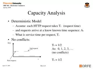
N(t) 2nd request t First request Capacity Analysis • Deterministic Model • Assume: each HTTP request takes Tr (request time) • and requests arrive at a know known time sequence: As • What is service time per request, Ts • No conflicts: Tr = 1/2 As: 0, 1, 2, 3, … (no conflicts) Ts = 1/2 Week 10
Round Robin N(t) 2nd request starts t Sequenced with conflict: • Round Robin: • Reqest 1 arrives at 0, works ‘till 0.25., waits ‘till .5 works ‘till .75 then ends • Reqest 2 arrives at.25, works ‘till 0.5., waits ‘till .75 works ‘till 1.0 then ends Ts = (0.75 + 0.75)/2 = 6/8 • First-come-first-serve Tr = 1/2 As: 0,.25, 1., 1.25,… (same # requests, sequenced differently) Ts = (0.5 + 0.75)/2 = 5/8 First request starts Week 10
Observations • If server is handling a single page, then deterministic service times is reasonable, otherwise NOT • The long term behavior depends on the arrival sequence, As, AND the service rate, Ts • F-C-F-S is a lower bound on the round robin Week 10
Probabilistic Model (F-C-F-S) • Let inter arrival time and the service times be : • independent, identically distributed (iid) random variables having an exponential distribution (denoted by M ) • a r.v. X has an exponential density iff: • f(x) = ae-ax x > 0 = 0 x < 0 So Prob{ X < x } = 1 - e-ax x > 0 Prob{ X > x } = e-ax x > 0 E(X) = 1/a var(X) = 1/a2 Week 10
l0 l1 ln Arrival Rates ... 0 1 2 n n+1 States mn+1 Service rates m1 m2 Assume server has been running for a while and reached steady state • In steady state (prob. of being in state j, (j waiting to be served)): Pjlj = Pj+1mj+1 or Pj+1 = Pj (lj /mj+1) (recursion relationship) Specifically: P1 = (l0 /m1) P0 P2 = (l1 /m2) P1 = (l1 /m2) (l0 /m1) P0 … Pn+1 = (ln /mn+1) Pn = ((ln ln-1 ...l0)/(mn+1 mn...m1)) P0 Let’s let: Cn = (ln-1 ln-2 ...l0)/(mn mn-1...m1) , n = 1, 2, … Then the Steady State Probabilities are Pn = Cn P0 , n = 1, 2, … Week 10
What about P0 ? • Since Sn=0, Pn = 1 , then Sn=0, Cn P0 = 1 P0 +Sn=1, Cn P0 = 1 P0 [1+Sn=1, Cn ]= 1 P0 = 1 / [1+Sn=1, Cn ] Now, the number of requests in the system, L L = 1 P1 +2 P2 +3 P3 +... = Sn=0, (n Pn ) Then the expected waiting time (likely time to be served),W = L /l laverage arrival time Week 10
Simple case: M/M/1/FCFS/ / Now suppose ln = l , mn = m , n = 1,2, 3, … then Cn= (ln / mn) = (l / m) n, n = 1,2, 3, … let r = l / m then P0 = 1 / (1 + Sn=1, rn)= 1 / Sn=1, rn ) Now recall Sn=1, xn = (1- xn+1 ) / (1- x) for any x and if |x| < 1 Sn=1, xn = 1/ (1- x) We need to have l < mor the system will blow up! So r < 1 Thus P0 = 1 / (1 / ( 1-r)) = 1 - r = 1 - (l / m) and Pn = rn P0 = rn ( 1-r) , n = 1,2, 3, … Week 10
What about L (expected # of requests in queuing system)? L = Sn=1, n Pn = Sn=1, n (1-r) rn = (1-r) Sn=1, n rn Now a little trick: Observe that n rn = n rrn-1 So L = (1-r) rSn=1, n rn-1 Why bother? Because n rn-1 should be familiar. In particulard/dr(rn ) = n rn-1 ThusL = (1-r) rSn=1, d/dr(rn ) = (1-r) r d/dr (Sn=1, (rn ) ) = (1-r) r d/dr (Sn=1, (rn ) ) but d/dr (Sn=1, inf (rn ) is a geometric series = (1-r) r d/dr(1-r )-1 , but d/dr(1-r )-1 = -1(1-r)-2 ( -1 ) So L = r(1- r )-1 and we can show L = l (m - l )-1 and expected time in system W = L / l = l (m - l )-1l-1 = (m - l )-1 Week 10
More of M/M/1/FCFS/ / Queues • Lq = expected number of customers in line = 0 P0 + Sn=1, ( n - 1) Pn = Sn=1, ( n Pn) - Sn=1, ( Pn) = L - (1 - P0 ) = L - r= l2 /(m (m - l )) • Ls = expected number of customers in service = 0 P0 + Sn=1, 1 Pn = 1 - P0 = 1 - (1 - r) = r= l / m • Wq = expected time of customer spends in line = Lq / l =l /(m (m - l )) • Ws = expected time of customer spends in service = Ls / l = 1 / m Week 10
What about multiple processors: Cn = (ln -1ln-2 ...l0)/(mnmn-1...m1) , n = 1, 2, … We again letln = l for every n Now assume that there are s processors. So when n < s we have mn = n m , and when n < s we have mn = s m So Cn = ln/(mn mn-1...m1) we has s terms of nm and n-s terms of sm Hence Cn = ln/ (n! mn) n < s = ln/ (s!)(sn-s) mn) n > s If l < s m as before we can show : Pn = 1/ ( Sn=0, s -1 {(1 / n! ) (l/ m )n + (1 / s! ) (l/ m )s )(1 - (l/ (s m)))} Week 10
Finally: Pn = P0 (l / m)n / (n!) n < s = P0 (l / m)n / ( (s!) sn-s )n > s L= P0 (l / m)s (l / s m) / ( s! ((1- l / s m)2 )) + l / m W= P0 (l / m)s (l / s m) / (l (s!) (1- (l / s m))2 )+ (1 +l ) / m Where L= s = # processors l = arrival rates m = processing rates Week 10
Realistic Server Performance • Consider one server connected to the internet Arrivals Initial processing “Server” Departures Browser Internet Model each as a single server queue Week 10
Arrivals Initial processing “Server” p Departures Browser Internet 1-p Realistic Server Performance, cont. • Assume: • File sizes are exponentially distributed • Service rate of browser and Internet are exponentially distributed • Parameters: • Arrival rate • Mean file size (5275 bytes) • Initialization time (independent of size) • Bandwidth @ Server (T1 = 1.5 Mbit/s , T3 = 6Mbit/s ) • Bandwidth @ Client (700Kbit/s) Response Time Arrival Rate 35/sec Week 10
“Server” “Server” More Complicated Model • Load balancing strategies (above not very smart) q Arrivals Initial processing 1-q p Departures Browser Internet 1-p Week 10