Low-Level Copy Number Analysis Part 1 - Background
Low-Level Copy Number Analysis Part 1 - Background. Henrik Bengtsson Post doc, Department of Statistics, University of California, Berkeley, USA CEIT Workshop on SNP arrays, Dec 15-17, 2008, San Sebastian. Acknowledgments. ISREC, Lausanne, Switzerland: Pratyaksha “Asa” Wirapati

Low-Level Copy Number Analysis Part 1 - Background
E N D
Presentation Transcript
Low-LevelCopy Number AnalysisPart 1 - Background Henrik Bengtsson Post doc, Department of Statistics, University of California, Berkeley, USA CEIT Workshop on SNP arrays, Dec 15-17, 2008, San Sebastian
Acknowledgments ISREC, Lausanne, Switzerland: • Pratyaksha “Asa” Wirapati Affymetrix, California: • Ben Bolstad • Simon Cawley • Steve Chervitz • Harley Gorrell • Earl Hubbell • Luis Jevons • Chuck Sugnet • Jim Veitch • Alan Williams UC Berkeley: • James Bullard • Kasper Hansen • Elizabeth Purdom • Terry Speed Lawrence Berkeley National Labs: • Amrita Ray • Paul Spellman John Hopkins, Baltimore: • Benilton Carvalho • Rafael Irizarry WEHI, Melbourne, Australia: • Mark Robinson • Ken Simpson
Detect more and smaller aberrations with less errors CRMA other #1 other #2 other #3 detection rate
Copy number analysis is about finding "aberrations" in one or several individuals
The HapMap project- Large project to identify SNPs in Humans (2003-) The HapMap is a catalog of common genetic variants (SNPs) that occur in human beings. It describes what These variants are, where they occur in our DNA, and How they are distributed among people within populations and among populations in different parts of the world. URL: http://www.hapmap.org/
The HapMap project- 270 normal individuals genotyped by different labs using various technologies • 90 CEU individuals (Utah/Europe, 30 trio families) • 90 YRI individuals (Nigeria; 30 trio families) • 45 CHB (China; unrelated) • 45 JPT (Japan; unrelated) Publicly available: • High quality data. • Raw data, e.g. Affymetrix CEL files. • Genotypes. • Studied by many groups.
Copy number polymorphism- People share common CN aberrations (2005-)
The Cancer Genome Atlas (TCGA) project- Large project for genetic mapping of tumors (2007-)
The TCGA project- A large number of tissues are studies with many DNA & RNA technologies • Tumor types: • brain cancer (glioblastoma multiforme, or GBM), • lung cancer (squamous cell carcinoma of the lung), and • ovarian cancer (serous cystadenocarcinoma of the ovary). • 234 tumors (of 500) characterized. • Multiple labs in the US • Broad, Harvard, Stanford, LBNL, … • High quality data. • Platforms: Affymetrix, Illumina, Agilent, … • Gene-, exon-, microRNA- expression, methylation, SNP & CN, sequencing… • Raw and summarized data immediately available (publicly), e.g. Affymetrix CEL files.
BACKGROUND: Whole-genome copy-number (CN) studies are rapidly expanding, and with this expansion comes a demand for increased precision and resolution of CN estimates. Several recent studies have obtained CN estimates from more than one platform on the same samples, and it is natural to want to combine the different estimates in order to meet this demand. PROBLEM: CN estimates from different platforms show different degrees of attenuation of the true CN changes. Differences can also be observed in CN estimates from the same platform run in different labs, or in the same lab, with different analytical methods. This is the reason why it is not straightforward matter to combine CN estimates from different sources (platforms, labs, analysis methods, etc). Combining copy numbers across platforms & labs Henrik Bengtsson (UC Berkeley), Amrita Ray (LBNL), Paul Spellman (LBNL), Terry Speed (UC Berkeley) (A) Broad, Affymetrix GWS6, n=1800K, 1.59kb/locus, 25-mers (B) Stanford, Illumina 550K, n=550K, 5.53kb/locus, 50-mers (C) MSKCC, Agilent 244K, n=236K, 12.7kb/locus, 60-mers (D) Harvard, Agilent 244K, n=236K, 12.7kb/locus, 60-mers Tumor/normal CNs by four TCGA centers (“sources”) in a 60Mb region on Chr3 in sample TCGA-02-104. (The combined set would consist of 2,822K loci with 0.95kb/locus.) The smoothed raw CNs from the four sources have similar CN profiles but different mean levels.
METHOD: We have developed a single-sample multi-source normalization that brings full-resolution CN estimates to the same scale across sources. Kernel estimators and principal component curves are used to estimate the non-linear relationships between the sources. Full-resolution data is then normalized such that these relationships become linear. The normalized estimates are such that for any underlying CN level, the mean level of the CN estimates is the same regardless of source. CNs with consistent mean levels are better suited for being combined across sources, e.g. existing segmentation methods may be used to identify aberrant regions. Before normalization: Non-linearity between pairs After normalization: Linearity between pairs Normalized full-resolution CNs for the four sources. The smoothed normalized CNs from the four sources have similar CN profiles and same mean levels.
(A) (B) (C) (D) (comb+raw) (comb+norm) At any given resolution (amount of smoothing), with combined normalized CNs (solid red) one can separate two CN states better than with combined raw CNs (dot-dashed red), and with each of the individuals sources (gray dotted). RESULTS: We use microarray-based CN estimates from The Cancer Genome Atlas (TCGA) project to illustrate the method. We show that after normalization the mean levels of randomly selected CN aberrations are the same across platforms, and that the normalized and combined data better separate two CN states at a given resolution. We conclude that it is possible to combine CNs from multiple sources such that the resolution becomes effectively larger, and when multiple platforms are combined, they also enhance the genome coverage by complementing each other in different regions. A 400kb region in TCGA-02-104 on Chr 3: CNs from different sources give different segmenting results at different precisions. With combined normalized CNs, there is more power to detect change points (CPs) and their locations are more precise.
* * * * 5 µm 5 µm 1 million identical 25-mer sequences The Affymetrix GeneChip is a synthesized high-density (single-array) microarray * 1.28 cm 1.28 cm 6.5 million probes/chip
* * * * * * * * * CN=1 CN=2 CN=3 PM = c PM = 2c PM = 3c Copy-number probes are used to quantify the amount of DNA at known loci CN locus:...CGTAGCCATCGGTAAGTACTCAATGATAG... PM:ATCGGTAGCCATTCATGAGTTACTA
Single Nucleotide Polymorphism (SNP) Definition: A sequence variation such that two chromosomes may differ by a single nucleotide (A, T, C, or G). Allele A:A ...CGTAGCCATCGGTA/GTACTCAATGATAG... Allele B:G A person is either AA, AB, or BB at this SNP.
* * * * * * * * * * * * * * * * * * * AA BB AB PMA >> PMB PMA << PMB PMA ¼PMB Probes for SNPs PMA:ATCGGTAGCCATTCATGAGTTACTA Allele A:...CGTAGCCATCGGTAAGTACTCAATGATAG...Allele B:...CGTAGCCATCGGTAGGTACTCAATGATAG...PMB:ATCGGTAGCCATCCATGAGTTACTA (Also MMs, but not in the newer chips, so we will not use these!)
* * * * * * * * * * * * * * * * * * * * * * * * AA AB AAB PM =PMA+PMB = 2c PM = PMA + PMB = 2c PM =PMA+PMB = 3c BB PM =PMA + PMB = 2c SNP probes can also be used toestimate total copy numbers *
The Affymetrix assay- takes 4-5 working days to complete • Start with target gDNA (genomic DNA) or mRNA. • Obtain labeled single-strandedtargetDNA fragments forhybridization to theprobeson the chip. • After hybridization, washing, and scanning we get a digital image. • Image summarized across pixels to probe-level intensities before we begin. This is our "raw data".
Restriction enzymes digest the DNA, which is then amplified and hybridized
Target DNA find their way to complementary probes by massive parallel hybridization
Image Analysis Example array: Dimensions: 1600x1600 cells Each cell: 3x3 pixels Dynamic range: 65536 (16-bits) intensity levels Cell summaries: (mean pixel, stddev pixel, #pixels)
Preparation + Hybridization + Scanning DAT File(s) [Image, pixel intensities] Image analysis CDF [Chip Description File] CEL File(s) [Probe Cell Intensity] + workable raw data Low-level analysis Segmentation
zoom in How did we get here? Data from 2003 on Chr22 (on of the smaller chromosomes)
Genome-Wide Human SNP Array 6.0- state-of-the-art array • > 906,600 SNPs: • Unbiased selection of 482,000 SNPs:historical SNPs from the SNP Array 5.0 (== 500K) • Selection of additional 424,000 SNPs: • Tag SNPs • SNPs from chromosomes X and Y • Mitochondrial SNPs • Recent SNPs added to the dbSNP database • SNPs in recombination hotspots • > 946,000 copy-number probes: • 202,000 probes targeting 5,677 CNV regions from the Toronto Database of Genomic Variants. Regions resolve into 3,182 distinct, non-overlapping segments; on average 61 probe sets per region • 744,000 probes, evenly spaced along the genome
4xfurther out… 10K 294kb 100K 26kb 500K 6.0kb # loci 5.0 3.6kb 6.0 1.6kb year Rapid increase in density Distance between loci: next? 2003 2004 2005 2006 2007
Affymetrix & Illumina are competing - we get more bang for the buck (cup) Price source: Affymetrix Pricing Information [http://store.affymetrix.com/] and Berkeley Coffee Shops, Dec 2008.
* * * * * * * * * * * 25 nucleotides Other DNA Other DNA Target seq. Other seq. X other PMs PM MM Affymetrix are moving away from MM probes- therefore we don’t utilize them Target DNA: ...CGTAGCCATCGGTAAGTACTCAATGATAG... ||||||||||||||||||||||||| Perfect match (PM): ATCGGTAGCCATTCATGAGTTACTA Mis-match (MM): ATCGGTAGCCATACATGAGTTACTA
Low-LevelCopy Number AnalysisPart 2 – Simple preprocessing Henrik Bengtsson Post doc, Department of Statistics, University of California, Berkeley, USA CEIT Workshop on SNP arrays, Dec 15-17, 2008, San Sebastian
* * * * * * * * * CN=1 CN=2 CN=3 PM = c PM = 2c PM = 3c Recap: Copy-number probes CN locus:...CGTAGCCATCGGTAAGTACTCAATGATAG... PM:ATCGGTAGCCATTCATGAGTTACTA
* * * * * * * * * * * * * * * * * * * * * * * * AA AB AAB PM =PMA+PMB = 2c PM = PMA + PMB = 2c PM =PMA+PMB = 3c BB PM =PMA + PMB = 2c Recap: Adding SNP probes gives total CN signal *
Notation- here and in our papers Indices: Arrays/samples: i = 1, 2, …, I Loci/SNPs/CN units: j = 1, 2, …, J Replicated probes for SNP: k = 1, 2, …, K Probe signals: CN locus: yij = PMij (single-probe units) SNP allele pair k: (yijkA,yijkB) = (PMijkA,PMijkB) Summarized signals (“chip effects”): CN locus: ij SNP: (ijA,ijB)
A simple way to obtain CN estimates • Calculate non-polymorphic SNP summaries: • For each array i=1,…,I and SNP j=1,…,J: • Probe allele pairs: (PMijkA,PMijkB); k=1,…,K • For both alleles, average across probes:ijA = mediank {PMijkA}, ijB = mediank {PMijkB} • Sum both alleles: ij = ijA + ijB • Calculate reference Rj across all arrays: • For each SNP j=1,…,J: • Rj = mediani {ij} • Calculate CN log-ratios: • For each array i=1,…,I and SNP j=1,…,J: • Mij = log2 (ij / Rj)
The software tools make this easy for you- using aroma.affymetrix package cs <- AffymetrixCelSet$byName(“GSE8605”, chipType=“Mapping10K_Xba142”); plm <- AvgCnPlm(cs, combineAlleles=TRUE); fit(plm); ces <- getChipEffectSet(plm); theta <- extractTheta(ces); thetaR <- rowMedians(theta); M <- log2(theta / thetaR);
Even without a segmentation algorithm, we can easily spot a deletion here. Copy number regions are found by lining up estimates along the chromosome Example: Log-ratios for one sample on Chromosome 22.
If we don’t add up the alleles, we get allele-specific estimates from which we can get genotypes Example: (ijA,ijB) for one SNPacross all samples BB AB AA
There are a lot of artifacts in microarray data- can we do better? Systematic variation can be added due to: • Spatial artifacts • Intensity dependent effects • Probe-sequence dependent effects • GC-content effects • PCR effects • Lab & people effects • Non-calibrated scanners • …?
Spatial artifacts (“extreme”) http://plmimagegallery.bmbolstad.com/
32.5Mb deletion on chr 11 = 0.246 Before = 0.225 After