Download
1 / 24
240 likes | 348 Vues
This retrospective analysis explores the evolution of models used to understand DNA sequences, focusing on finite state automata and Hidden Markov Models (HMMs). It discusses the limitations of deterministic models in representing complex biological states, emphasizing the need for probabilistic frameworks like HMMs. Various topologies of HMMs are presented, highlighting their flexibility to accommodate different state duration distributions and effectively model bioinformatics problems. The paper underscores the importance of state transitions and emissions in capturing sequence dynamics, including handling gaps and mutations.

E N D
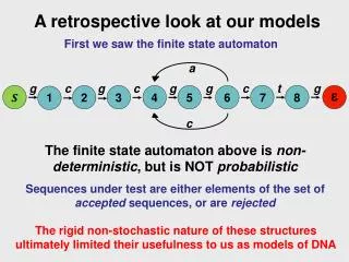
A retrospective look at our models First we saw the finite state automaton a g c g c g g c t g e S 1 2 3 4 5 6 7 8 c The finite state automaton above is non-deterministic, but is NOT probabilistic Sequences under test are either elements of the set of accepted sequences, or are rejected The rigid non-stochastic nature of these structures ultimately limited their usefulness to us as models of DNA
States Transition probabilities Markov Model What do we need to probabilistically model DNA sequences? A C T G Here each observation necessarily corresponded to the underlying biological state…which also limited the usefulness and generality of the concept as a model for DNA or amino acid sequences
HMM Topology Many different HMM topologies are possible… a R e S b Careful selection of alternative HMM topologies will allow us to address a variety of different problems using essentially the same algorithmic toolkit
HMM Topology Duration modeling with HMMs CpG+ e S p CpG - Consider our CpG island model with two underlying states…. How long does our model dwell in a particular state? P(L residues) = (1-p)·pL-1 This should be familiar as an exponentially decaying value
HMM Topology Duration modeling with HMMs CpG+ e S p CpG - P P(L residues) = (1-p)·pL-1 L What if this doesn’t accurately reflect the real distribution of lengths?
HMM Topology Duration modeling with HMMs etc. etc. Assuming that each state shown here has the same emission frequencies, this forms an example of a submodel topology that will guarantee a minimum of four symbols drawn from the same underlying emission distribution, but with a length distribution that is still geometric. The duration of the model has been tweaked. There are many more complex possibilities depending on the properties of the length distribution you seek to model Note: this and numerous other figures that follow in this presentation are after Durbin et al.
HMM Topology etc. Duration modeling with HMMs etc. The topology shown in this variation can model any desired distribution of lengths varying between 2 and 6
HMM Topology Duration modeling with HMMs p p p p etc. etc. 1-p 1-p 1-p 1-p Where n = number of repetitive states, so here n = 4 Without belaboring the derivation, we’ll just mention that this negative binomial distributionoffers a great deal of flexibility in modeling length distributions
HMM Topology Duration modeling with HMMs http://www.boost.org/doc/libs/1_40_0/libs/math/doc/sf_and_dist/html/ math_toolkit/dist/dist_ref/dists/negative_binomial_dist.html By selecting appropriate values for the number of repeating states and the probability of re-entering each state, you can flexibly model the length distribution
HMM Topology Duration modeling with HMMs http://www.boost.org/doc/libs/1_40_0/libs/math/doc/sf_and_dist/html/ math_toolkit/dist/dist_ref/dists/negative_binomial_dist.html http://www.boost.org/doc/libs/1_40_0/libs/math/doc/sf_and_dist/html/ math_toolkit/dist/dist_ref/dists/negative_binomial_dist.html In practical HMMs we would probably use n much smaller than in these examples, but with probability of state re-entry much closer to 1
HMM Topology A trivial HMM is equivalent to a Position Specific Scoring Matrix The transitions are deterministic and Pr{aMi→Mi+1}= 1 but the emissions correspond to the estimated amino acid or nucleotide frequencies in the columns of a PSSM . . . e S M1 M2 ML We refer collectively to M1…Mj as match states This simple model cannot account for indelsand does not capture all of the information present in a multiple alignment
HMM Topology Insertions are handled with special states with background-like emission Ij . . . e S M1 Mj Mj+1 Insertion states correspond to states that do not match anything in the model. They almost always have emission probabilities matching the background distribution We still need a way to deal with deletions…
HMM Topology How do insertions affect the overall probability of a sequence? For an insertion of length k: Ij . . . e S M1 Mj Mj+1 log aMj→Ij+ (k-1)·log aIj→Ij + log aIj→Mj+1 Assuming log-odds scoring relative to some background distribution, emissions from Ij will not contribute to the overall score, and only the transitions will matter
HMM Topology How do insertions affect the overall probability of a sequence? For an insertion of length k: Ij . . . e S M1 Mj Mj+1 log aMj→Ij+ (k-1)·log aIj→Ij + log aIj→Mj+1 This is equivalent to the familiar gap opening+gap extension penalties used in many sequence alignment methods. This is therefore a form of affine gap scoring
HMM Topology How best to handle deletions? e S The problem with allowing arbitrarily long gaps in any practically sized model is that we would need to estimate far too many transition probabilities Estimation is the hardest HMM problem, so we should avoid an unnecessary proliferation of transitions wherever possible!
HMM Topology In general we handle deletionsby adding silent states… Dj e S Mj We can use a sequence of silent-state transitions to move from any match state to any other match state! Note that not all Dj→Dj+1 transitions need have the same probability
The Profile HMM If we combine all these features, we have the famous profile HMM Dj Ij e S Mj We can use a sequence of silent-state transitions to move from any match state to any other match state! Profile HMMs fully generalise the concept of pairwise alignment!
The Profile HMM If we combine all these features, we have the famous profile HMM Dj Ij e S Mj Profile HMMs are extensively used for the identification of new members of conserved sequence families This relies on the ability to estimate parameters for the profile HMM on the basis of multiple sequence alignments
Basic estimation for profile HMMs Consider a multiple sequence alignment #pos 01234567890 >glob1 VGA--HAGEY >glob2 V----NVDEV >glob3 VEA--DVAGH >glob4 VKG------D >glob5 VYS--TYETS >glob6 FNA--NIPKH >glob7 IAGADNGAGV *** ***** First heuristic: positions with more than 50% gaps will be modeled as inserts, the remainder as matches. In this example only the starred columns will correspond to matches We can now count simply count the transitions and emissions to calculate our maximum likelihood estimators from frequencies. But what about missing observations?
Basic estimation for profile HMMs Parameter estimation from multiple alignments Second heuristic: use pseudocounts to fill in missing observations.. Here B is the total number of pseudocounts, and q represents the fraction of the total number that have been allocated to that particular transition or emission Let’s start by simply applying Laplace’s rule: add one pseudocount to every frequency calculation
Basic estimation for profile HMMs Consider a multiple sequence alignment #pos 01234567890 >glob1 VGA--HAGEY >glob2 V----NVDEV >glob3 VEA--DVAGH >glob4 VKG------D >glob5 VYS--TYETS >glob6 FNA--NIPKH >glob7 IAGADNGAGV *** ***** eM1(V) = 6/27, eM1(I) = eM1(F) = 2/27, eM1(all other aa) = 1/27 aM1→M2 = 7/10, aM1→D2 = 2/10, aM1→I1= 1/10, etc. These are the estimates when we apply Laplace’s rule for adding pseudocounts..
Scoring with profile HMMs The state path of sequences under test are always unknown • Since the state path is unknown we have two basic options: • Employ the Viterbi algorithm to determine the joint probability of the observed sequence and the most probable state path • Employ the forward (or backward) algorithm to determine the full probability summed over all possible state paths Either way, one fly in the ointment is that we are usually interested in a score expressed as a log-odds ratio relative to our random model: We could calculate separate scores for the models, then combine, but this is inefficient
Scoring with profile HMMs Modifying Viterbi and Forward for profile HMMs We could rewrite the recurrences to accommodate log-odds scoring. For example, Viterbi might look like this: This would be a serious nuisance except we already have a log_float class!!! So, we can instead just alter our emission terms to the form below: emission = log_float() In other words, we need only adjust and “log_floatize” our emissions, which is something we can do up front in the self.emissionsdict rather than in the algorithms
Handling multiple sequences in Python Inheritance is a powerful tool for deriving new classes class FastA(list): # note derivationfromlist, not object def __init__(self): #stuff defread_file(self, filepath): # stuff defcalculate_MLE(self, pseudocounts) # stuff return (transitions, emissions) Our goal is to develop a class, FastA, that behaves like a python list that serves as a container for sequences read from a file. Each element will contain a tuple of the annotation and the sequence stored as a string. It should also be able to use these sequences to then calculate “dict-of-dict” transition and emission distributions suitable for use in our increasingly sophisticated HMM class I’ll provide more information about the key methods in the form of a Python docstring