High Gain Observer
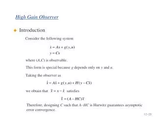
High Gain Observer. Introduction. Consider the following system. where ( A , C ) is observable. This form is special because g depends only on y and u. Taking the observer as. we obtain that satisfies.

High Gain Observer
E N D
Presentation Transcript
High Gain Observer • Introduction Consider the following system where (A,C) is observable. This form is special because g depends only on y and u. Taking the observer as we obtain that satisfies Therefore, designing C such that AHC is Hurwitz guarantees asymptotic error convergence.
High Gain Observer (Continued) However, any error in modeling g will be reflected in the estimation error equation. Thus, where is a nominal model of g. Hence We give a special design of the observer gain that makes the observer robust to uncertainties in modeling the nonlinear functions. The technique, called as high-gain observers, works for a wide class of nonlinear systems and guarantees that the output feedback controller recovers the performance of the state feedback controller when the observer gain is sufficiently high.
High Gain Observer (Continued) The main result is a separation principle that allows us to separate the design into two tasks. First, design a state feedback controller that stabilizes the system and meets other design specifications. Then, obtain an output feedback controller by replacing x by provided by the high-gain observer. A key property that makes this separation possible is the design of the state feedback controller to be globally bounded in x.
Example Ex: Assume that u = (x) is a local state feedback control law that stabilizes the origin. To implement this control law using only y, we use the observer where is a nominal model of the nonlinear function Then where
Example (Continued) We want to design such that In the absence of , asymptotic error convergence is achieved by designing H such that is Hurwitz. In the presence of , we need to design H with the goal of rejecting the effect of on This is ideally achieved, for any , if the transfer function from to is ideally zero.
Example (Continued) While this is impossible, we can make arbitrarily small by choosing Taking it can be shown that Hence Define the scaled estimation errors Then the newly defined variables satisfy the singularly perturbed equation. This equation shows clearly that reducing diminishes the effect of .
Example (Continued) Notice, however, that will be whenever Consequently, the solution contains a term of In fact, This behavior is known as the peaking phenomenon.
Globally Stabilized by State Feedback Controller Let’s consider the system which can be globally stabilized by the state feedback controller The output controller is taken as where the observer gain assigns the eigen values of
State Feedback Controller The above figure shows a counter intuitive behavior as 0. Since decreasing causes the estimation error to decay faster toward zero, one would expect the response under output feedback to approach the response under state feedback as decreases. This is the impact of peaking phenomenon. Fortunately, we can overcome the peaking phenomenon by saturating the control outside a compact region of interest in order to create a buffer that protects the plant from peaking.
State Feedback Controller Suppose the control is saturated as The above figure shows the performance of the system under saturated state and output feedback. The control u is shown on a shorter time interval that exhibits control saturation during peaking. The peaking period decreases with .
Stabilization Consider the MIMO nonlinear system (1)
Output Feedback Controller The functions , and q are locally Lipschitz and (0,0,0)=0, (0,0,0)=0, q(0,0)=0. Our goal is to find an output feedback controller to stabilize the origin. We use a two-step approach to design the output feedback controller. (i) A partial state feedback controller using x and is designed to asymptotically stabilize the origin. (ii) A high-gain observer is used to estimate x from y. The state feedback controller can be shown as where r, are locally Lipschitz in their arguments over the domain of interest and globally bounded functions of x. Moreover, r(0,0,0)=0 and (0,0,0)=0.
Output Feedback Controller (Continued) For convenience, we write the closed-loop system under state feedback as (2) where X = (x, z, ). The output controller is taken as (3)
Output Feedback Controller (Continued) The observer gain H is chosen as
Theorem: Consider the closed-loop system of the plant (1) and the output feedback controller (3). Suppose the origin of (2) is asymptotically stable and R is its region of attraction. Let S be any compact set in the interior of R and Q be any compact subset of Then, Theorem
Theorem (Continued) (2), (2) Proof: See Ch 14.5
Results The theorem shows that the output feedback controller recovers the performance of the state feedback controller for sufficiently small . Note that (i) recovery of exponential stability (ii) recovery of the region of attraction in the sense that we can recover any compact set in its interior (iii) the solution under output feedback approaches the solution under the state feedback as 0.
Example Ex: Consider the following plant: Note : the given system is in triangular form. Thus, it is stabilizable by The output feedback controller is
Example (Continued) with For simulation: All system eigenvalues at 5. All observer eigenvalues at 5/ with = 0.05.