Understanding Depth-First Search in Image Analysis and Graph Traversal
Depth-First Search (DFS) is an essential algorithm in image analysis and graph traversal. It identifies regions in digital images represented as arrays of pixels, facilitating the grouping of contiguous pixels with the same value. The algorithm recursively explores unvisited neighbors to uncover regions, retreating when necessary. Additionally, DFS can be applied to graphs, treating pixels as vertices and shared edges as adjacency. The approach is efficient, with a time complexity of Θ(m+n). This foundational method is pivotal for applications in computer graphics and data structure algorithms.

Understanding Depth-First Search in Image Analysis and Graph Traversal
E N D
Presentation Transcript
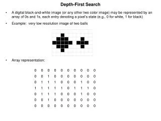
Depth-First Search • A digital black-and-white image (or any other two color image) may be represented by an array of 0s and 1s, each entry denoting a pixel’s state (e.g., 0 for white, 1 for black) • Example: very low resolution image of two balls • Array representation:
Depth-First Search • One of the important steps in image analysis is to identify its regions – groups of contiguous pixels with the same value • The neighbors of a pixel are defined to be those to the left, up, right and down directionsN N P N N • One method proceeds as follows. If we are at a pixel p with value v: • if p has an unvisited neighbor with the same value, go to one of these neighbors and continue from there; • if there are no unvisited neighbors with the value v and p is not the initial pixel of our search, we retreat to the pixel from which we first visited p and try to find another one of its unvisited, same-value neighbors • If p is the initial pixel and has no unvisited neighbors with the same value, we start a new search at an unvisited pixel with value v. • This method is known as depth-first search and has a wide variety of applications
Depth-First Search on Graphs • A digital image may be represented as a graph as follows • Replace each pixel with a vertex • Two vertices are adjacent if the associated pixels share an edge • Depth-first search may be extended to arbitrary graphs • The generic recursive depth-first search function is as follows: • void dfs(v) { for each vertex w adjacent to v { if w is unvisited { visit w; /* mark w as visited and do any other desired processing */ dfs(w); } }
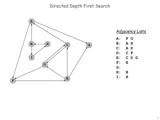
We illustrate the DFS algorithm execution with the following graph We assume that we process the adjacent vertices of our current vertex in alphabetical order. Our initial call will be dfs(a,…).
dfs(a) dfs(e)
dfs(a) dfs(e) dfs(b)
dfs(a) dfs(e)
dfs(a) dfs(e) dfs(c)
dfs(a) dfs(e) dfs(c) dfs(d)
dfs(a) dfs(e) dfs(c) dfs(d) dfs(g)
dfs(a) dfs(e) dfs(c) dfs(d) dfs(g) dfs(f)
dfs(a) dfs(e) dfs(c) dfs(d) dfs(g)
dfs(a) dfs(e) dfs(c) dfs(d)
dfs(a) dfs(e) dfs(c) dfs(d) dfs(h)
dfs(a) dfs(e) dfs(c) dfs(d) dfs(h) dfs(i)
dfs(a) dfs(e) dfs(c) dfs(d) dfs(h) dfs(i) dfs(j)
dfs(a) dfs(e) dfs(c) dfs(d) dfs(h) dfs(i)
dfs(a) dfs(e) dfs(c) dfs(d) dfs(h)
dfs(a) dfs(e) dfs(c) dfs(d)
dfs(a) dfs(e) dfs(c)
dfs(a) dfs(e)
DFS Code • Input parameters: adj, start, visit Output parameters: none • dfs( adj, start ) { n = adj.last // number of nodes in the graph for i = 1 to n visit[i] = false dfs_recurs( adj, start, visit )} • dfs_recurs( adj, w,visit ) {println(w) visit [w] = true trav = adj[w] // pointer to first node of adjacency list of w while ( trav != null ) { v = trav.ver // a vertex adjacent to w if ( !visit[v] ) dfs_recurs( adj, v, visit ) // continue searching from v trav = trav.next // after finishing dfs(v), go to the next vertex adj to w }}
Running Time of DFS • Suppose that a graph with m edges and n vertices is input to the dfs algorithm • The for-loop in dfs runs in time (n) • After dfs calls dfs_recurs, the worst case is where every vertex in every adjacency list examined. Since there are 2m vertex occurrences in the adjacency lists, the total time for all the calls to dfs_recurs is (m) • Thus the total worst-case running time for dfs is (m+n)
Connectedness using DFS • Input parameters: adj Output parameters: none • is_connected( adj ) { n = adj.last for i = 1 to n visit[i] = false dfs_recurs(adj,1, visit) for i = 1 to n if ( !visit[i] ) return false return true}
DFS Orientation of an Undirected Graph • We can use dfs to turn an undirected graph G into a directed graph • During dfs, each edge {u,v} is examined in each of the two possible directions • Once when we are executing dfs(u) and again when we are doing dfs(v) • The orientation algorithm assigns the direction that was an edge was first examined. • We call the result a dfs orientation of G. • The algorithm has the following property: • If G is connected and has no edges whose removal disconnects G, then every dfs orientation of G is strongly connected.
DFS Orientation of an Undirected Graph • dfs_orient( adj, start, D ) { n = adj.last // number of nodes in the graph for i = 1 to n visit[i] = false for j = 1 to n D[i][j] = 0 // initially edgeless directed graph dfs_recurs( adj, start )} • dfs_orient_recurs( adj, w, visit, D ) { visit [w] = true trav = adj[w] // pointer to first node of adjacency list of w while ( trav != null ) { v = trav.ver // a vertex adjacent to w if D[v][w] == 0 // this is the first time we have looked down the edge D[w][v] = 1 if ( !visit[v] ) dfs_orient_recurs( adj, v, visit, D ) // continue searching from v trav = trav.next }}
Homework • Pages 179-180: # 2, 3, 9 • Draw the orientation produced by the example execution of dfs in these slides (see slide 4).