Download

1 / 17
170 likes | 324 Vues
Calculating the entropy on-the-fly. Daniel Lewandowski Faculty of Information Technology and Systems, TU Delft. Introducing a function h. h - is a measure of the uncertainty about the outcome of an experiment modelled using probability distributions. Assumptions. We assume that h :

E N D
Calculating the entropy on-the-fly Daniel Lewandowski Faculty of Information Technology and Systems, TU Delft
Introducing a function h. h - is a measure of the uncertainty about the outcome of an experiment modelled using probability distributions
Assumptions • We assume that h: • depends only on the probability of the outcome of an experiment or event • takes values in non-negative real numbers • is a continuous and decreasing function • h(p1p2)=h(p1)+h(p2) The assumptions forces h to be of the form: h(p)= - C log(p)
Definition of entropy The entropy H is the expectation of the function h. Example: x1, x2,…,xnare realizations of a rand. variab. X with probabilities p1, p2,…,pn respectively. Then the entropy of X is:
Units in which the entropy is measured log2(x) – bits log3(x) – trits ln(x) – nats log10(x) – Hartleys
Entropy of some continuous distributions • The standard normal (Gaussian) distribution: H = 1,4189 • The Weibull distribution (=1,127; =2,5): H = 0,5496 • The Weibull distribution (=1,107; =1,5): H = 0,8892 • The gamma distribution (==5): H = 0,5441
Approximation of the density Y1,Y2,…,Yn – samples D0,D1,…,Dn – midpoints D0=Y1 – (Y2 – Y1)/2, Di=Yi+1 – (Yi+1 – Yi)/2, for i=2,…,n-1 Dn=Yn + (Yn – Yn-1)/2,
Computations The density above the Yi is estimated as: The entropy is then computed as:
Grouping samples Remark: The result of calculating the entropy without grouping samples is biased – the bias is asymptotically equal to - 1 + ln2, ( - Euler constant)
Numerical test – 5000 samples Entropy 1,159 1,372 1,399 1,458 1,438 1,418 1,324 Exact : 1,418 The red line marks the exact density function of a standard normal vrb.
Results – 20 iterations (1000 samples) Compare results to exact solutions from slide 6
Updating the distribution before updating after updating Dk Dk+1 Dk+2 Yk Yk+1 D(N+1) Y(N+1) D(N+2)
Updating the entropy HN – the entropy calculated based on N samples. where:
The program - properties • Uses the approach from the previous slide • Starts updating the entropy from N=4 • Written in VBA, uses spreadsheet only to store the samples • Results exactly the same as computed in Matlab (for the same samples) • It is not grouping samples
Results Comparison of results obtained using formula and program (5000 samples – without grouping and adding the bias). The program updates the entropy HN starting from N = 4.