Download
1 / 25
250 likes | 360 Vues
22. 22. 9. 13. 7. 15. 6. 7. 4. 3. 6. 9. 4. 3. Cost = 42. Cost = 44. Best merge order?. Optimal Merging Of Runs. 22. 7. 15. 4. 3. 6. 9. Weighted External Path Length. WEPL(T) = S (weight of external node i) * (distance of node i from root of T).

E N D
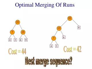
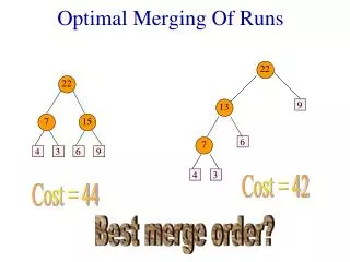
22 22 9 13 7 15 6 7 4 3 6 9 4 3 Cost = 42 Cost = 44 Best merge order? Optimal Merging Of Runs
22 7 15 4 3 6 9 Weighted External Path Length WEPL(T) = S(weight of external node i) * (distance of node i from root of T) • WEPL(T) = 4 * 2 + 3*2 + 6*2 + 9*2 • = 44 = Merge Cost
22 13 7 9 6 4 3 Weighted External Path Length WEPL(T) = S(weight of external node i) * (distance of node i from root of T) • WEPL(T) = 4 * 3 + 3*3 + 6*2 + 9*1 • = 42 = Merge Cost Find binary tree with minimum WEPL.
Other Applications • Message coding and decoding. • Lossless data compression.
Message Coding & Decoding • Messages M0, M1, M2, …, Mn-1 are to be transmitted. • The messages do not change. • Both sender and receiver know the messages. • So, it is adequate to transmit a code that identifies the message (e.g., message index). • Mi is sent with frequency fi. • Select message codes so as to minimize transmission and decoding times.
Example • n = 4 messages. • The frequencies are [2, 4, 8, 100]. • Use 2-bit codes [00, 01, 10, 11]. • Transmission cost = 2*2 + 4*2 + 8*2 + 100*2 = 228. • Decoding is done using a binary tree.
0 1 0 1 2 4 8 100 M0 M1 M2 M3 Example • Decoding cost = 2*2 + 4*2 + 8*2 + 100*2 = 228 = transmission cost = WEPL
0 1 100 M3 0 1 8 M2 0 1 2 4 M0 M1 Example • Every binary tree with n external nodes defines a code set for n messages. • Decoding cost • = 2*3 + 4*3 + 8*2 + 100*1 • = 134 • = transmission cost • = WEPL
1 0 0 1 0 1 0 1 0 M9 0 1 1 M4 M5 M8 M6 M7 M0 M1 M2 M3 Another Example No code is a prefix of another!
Lossless Data Compression • Alphabet = {a, b, c, d}. • String with 10 as, 5 bs, 100 cs, and 900 ds. • Use a 2-bit code. • a = 00, b = 01, c = 10, d = 11. • Size of string = 10*2 + 5*2 + 100*2 + 900*2 = 2030 bits. • Plus size of code table.
Lossless Data Compression • Use a variable length code that satisfies prefix property (no code is a prefix ofanother). • a = 000, b = 001, c = 01, d = 1. • Size of string = 10*3 + 5*3 + 100*2 + 900*1 = 1145 bits. • Plus size of code table. • Compression ratio is approx. 2030/1145 = 1.8.
Lossless Data Compression 0 1 • Decode 0001100101… • addbc… • Compression ratio is maximized when the decode tree has minimum WEPL. d 0 1 c 0 1 a b
Huffman Trees • Trees that have minimum WEPL. • Binary trees with minimum WEPL may be constructed using a greedy algorithm. • For higher order trees with minimum WEPL, a preprocessing step followed by the greedy algorithm may be used. • Huffman codes: codes defined by minimum WEPL trees.
Greedy Algorithm For Binary Trees • Start with a collection of external nodes, each with one of the given weights. Each external node defines a different tree. • Reduce number of trees by 1. • Select 2 trees with minimum weight. • Combine them by making them children of a new root node. • The weight of the new tree is the sum of the weights of the individual trees. • Add new tree to tree collection. • Repeat reduce step until only 1 tree remains.
2 5 4 7 9 9 Example • n = 5, w[0:4] = [2, 5, 4, 7, 9].
Example • n = 5, w[0:4] = [2, 5, 4, 7, 9]. 5 5 7 7 9 9 6 2 4
6 Example • n = 5, w[0:4] = [2, 5, 4, 7, 9]. 7 9 11 5 2 4
2 7 5 4 9 6 Example • n = 5, w[0:4] = [2, 5, 4, 7, 9]. 11 16
2 7 5 16 27 4 9 6 Example • n = 5, w[0:4] = [2, 5, 4, 7, 9]. 11
Data Structure For Tree Collection • Operations are: • Initialize with n trees. • Remove 2 trees with least weight. • Insert new tree. • Use a min heap. • Initialize … O(n). • 2(n – 1) remove min operations … O(n log n). • n – 1 insert operations … O(n log n). • Total time is O(n log n). • Or, (n – 1) remove mins and (n – 1) change mins.
6 6 3 3 4 10 19 19 9 1 1 9 Optimal Tree Cost = 23 Higher Order Trees • Greedy scheme doesn’t work! • 3-way tree with weights [3, 6, 1, 9]. Greedy Tree Cost = 29
10 Greedy Tree Cost = 29 6 3 19 1 9 0 Cause Of Failure • One node is not a 3-way node. • A 2-way node is like a 3-way node, one of whose children has a weight of 0. • Must start with enough runs/weights of length 0 so that all nodes are 3-way nodes.
How Many Length 0 Runs To Add? • k-way tree, k > 1. • Initial number of runs is r. • Add least q >= 0 runs of length 0. • Each k-way merge reduces the number of runs by k – 1. • Number of runs after sk-way merges is r + q – s(k – 1) • For some positive integer s, the number of remaining runs must become 1.
How Many Length 0 Runs To Add? • So, we want r + q – s(k–1) = 1 for some positive integer s. • So, r + q – 1 = s(k – 1). • Or, (r + q – 1) mod (k – 1) = 0. • Or, r + q – 1 is divisible by k – 1. • This implies that q < k – 1. • (r – 1) mod (k – 1) = 0 => q = 0. • (r – 1) mod (k – 1) != 0=> q = k –1 –(r – 1) mod (k – 1). • Or, q =(1 – r) mod (k – 1).
Examples • k = 2. • q =(1 – r) mod (k – 1) = (1 – r) mod 1 = 0. • So, no runs of length 0 are to be added. • k = 4, r = 6. • q =(1 – r) mod (k – 1) = (1 – 6) mod 3 = (–5)mod 3 = (6 – 5) mod 3 = 1. • So, must start with 7 runs, and then apply greedy method.