Streamflow and Climate Reconstruction Methodology Explained

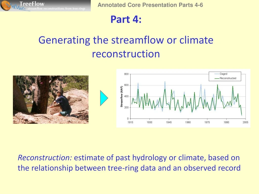
1. Annotated Core Presentation Parts 4-6 Part 4: Generating the streamflow or climate reconstruction Reconstruction: estimate of past hydrology or climate, based on the relationship between tree-ring data and an observed record

2. Overview of reconstruction methodology Tree Rings (predictors) Observed Flow/Climate (predictand) Statistical Calibration Reconstruction Model Model validation Streamflow/climate reconstruction Adapted from graphic by David Meko

3. Requirements: Tree-ring chronologies • Moisture sensitive species • Location • – From a region that is climatically linked to the gage of interest • Because weather systems cross watershed divides, chronologies do not have to be in same basin as gage • Length • Last year close to present for the longest calibration period possible • First year as early as possible (>300 years) but in common with a number of chronologies • Significant correlation with observed record

4. Requirements: Observed streamflow/climate record • Length – minimum 40 years in common with tree-ring data for robust calibration • Natural/undepleted record – flows must be corrected for depletions, diversions, evaporation, etc. • Homogeneous (climate record) – inspected for station moves, changes in instrumentation Fraser River at Winter Park Undepleted Flow (from Denver Water) USGS Gaged Flow The reconstruction quality relies on the quality of the observed record.

5. Tree Rings (predictors) Observed Flow/Climate (predictand) Statistical Calibration Reconstruction modeling strategies • Tree-ring data are calibrated with an observed streamflow record to generate a statistical model • Individual chronologies are used as predictors (dependent variables) in a statistical model, or • A set of chronologies is reduced through averaging or Principal Components Analysis (PCA), and the average or principal components (representing modes of variability) are used as predictors in a statistical model • Most common statistical method: Linear Regression • Other approaches: neural networks • Alternative: Non-Parametric method uses the relationships within the tree-ring data set to resample years from the observed record

6. Model validation and skill assessment • Are regression assumptions satisfied? • How does the model validate on data not used to calibrate the model? • How does the reconstruction compare to the gage record?

7. Calibration Validation How does the model validate on data not used to calibrate the model? Split-sample with independent calibration and validation periods Cross-validation: “leave-one-out” method, iterative process Calibration/validation

8. Calibration Validation R2 Gage RE Boulder Creek at Orodell 0.65 0.60 Rio Grande at Del Norte 0.76 0.72 Colorado R at Lees Ferry 0.81 0.76 Gila R. near Solomon 0.59 0.56 Sacramento R. 0.81 0.73 Two statistics for model assessment • Calibration: Explained variance: R2 • Validation: Reduction of Error (RE): model skill compared to no knowledge (e.g., the calibration period mean) What are desirable values? Of course, higher R2s are best, and positive value of RE indicates some skill (the closer to R2 the better)

9. How does the reconstruction compare to the gage record? Observed vs. reconstructed flows - Lees Ferry The means are the same, as expected from the the linear regression Also as expected, the standard deviation (variance) in the reconstructionis lower than in the gage record

10. Subjective assessment of model quality • Are severe drought years replicated well, or at least correctly classified as drought years? • Wet years?

11. Subjective assessment of model quality • Are the lengths and total deficits of multi-year droughts replicated reasonably well?

12. From model to full reconstruction When the regression model has been fully evaluated, the model is applied to the full period of tree-ring data to generate the reconstruction Tree Rings (predictors) Observed Streamflow (predictand) Statistical Calibration Reconstruction Model Model validation

13. Part 5: Uncertainty in the reconstructions

14. Sources of uncertainty in reconstructions • Observed streamflow and climate records contain errors • Trees are imperfect recorders of climate and streamflow, and the reconstruction model will never explain all of the variance in the observed record (“model error”) • A number of decisions are made in the modeling process, all of which can have an effect on the final reconstruction (“model sensitivity”)

15. Using the model error to generate confidence intervals for the reconstruction Colorado R. at Lees Ferry • Gray band = 95% confidence interval around reconstruction (derived from mean squared error, RMSE) • Indicates 95% probability that the observed flow falls within the gray band

16. Application of model error: using RMSE-derived confidence interval in drought analysis Lees Ferry Reconstruction, 1536-19975-Year Running MeanAssessing the 2000-2004 drought in a multi-century context Data analysis: Dave Meko

17. An alternative approach to generate confidence intervals on the reconstruction • “Noise-added” reconstruction approach • A large number of plausible realizations of true flow from derived from the reconstructed values and their uncertainty allow for probabilistic analysis. One of 1000 plausible ensemble of “true” flows, which together, can be analyzed probabilistically for streamflow statistics Meko et al. (2001)

18. Sensitivity of the reconstruction to choices made in the reconstruction modeling process • the calibration record used • the span of years used for the calibration • the selection of tree-ring data • the treatment of tree-ring data • the statistical modeling approach used • There is usually no clear “best” model

19. Sensitivity to calibration period South Platte at South Platte, CO Annual Flow (MAF) Calibration data ––– Standard Model ––– Ensemble Mean ––– Ensemble Members ––– • Each of the 60 traces is a model based on a different calibration period • All members have similar sets of predictors

20. Sensitivity to available predictors • How sensitive is the reconstruction to the specific predictor chronologies in the pool and in the model? Animas River at Durango, CO – two independent models Best stepwise model R2 = 0.82 Alternate stepwise model - predictors from best model excluded from pool R2 = 0.79

21. Alternate 1,200,000 Best-fit 1,000,000 800,000 600,000 400,000 200,000 0 1500 1550 1600 1650 1700 1750 1800 1850 1900 1950 2000 Sensitivity to available predictors Animas River at Durango, CO - two independent reconstructions • The two models correlate at r = 0.89 over their overlap period, 1491-2002 • Completely independent sets of tree-ring data resulted in very similar reconstructions

22. Sensitivity to other choices made in modeling process Lees Ferry reconstructions from 9 different models that vary according to chronology persistence, pool of predictors, modeling strategy Lees Ferry Reconstructions, 20-yr moving averages Analysis from David Meko

23. Lees Ferry reconstructions, generated between 1976 and 2007 Differences due to combinations of all of the factors mentioned calibration 20-year running means Stockton-Jacoby (1976), Michaelson (1990), Hidalgo (2001),Woodhouse (2006), Meko (2007)

24. Uncertainty related to extreme values Colorado at Lees Ferry, Reconstructed and Gaged Flows Extremes of reconstructed flow beyond the gaged record often reflect tree-ring data outside the calibration space of the model

25. Uncertainty summary • We can measure the statistical uncertainty due to the errors in the reconstruction model, but this does not fully reflect uncertainty resulting from sensitivity to model choices • There are other ways to estimate reconstruction uncertainty or confidence intervals (i.e. Meko et al. “noise added” approach) • For a given gage, there may be no one reconstruction that is the “right one” or the “final answer” • Some reconstructions may be more reliable than others (model validation assessment, length of longer calibration period, better match of statistical characteristics of the gage record) • ►A reconstruction is a plausible estimate of past streamflow

26. Part 6: What reconstructions can tell us about droughts of the past

27. Colorado River: The 20th century contains only a sample of the interannual variability of the last 500 years

28. Rio Grande: The extreme low flows of the past 100 years (like 2002) were exceeded prior to 1900 2002 • Gage record in blue, reconstruction in green • 5 reconstructed annual flows before 1900 were likely to have been lower than 2002 gaged flow (1685, 1729, 1748, 1773, 1861)

29. Rio Grande: Multi-year droughts were clustered in time, with fewer droughts in the 20th century Reconstructed Rio Grande Streamflow, 1536-1999 Periods of below-average flow, of 2 years or more (length of bar shows acre-feet below average)

30. Rio Grande: The longest observed droughts are exceeded in length by pre-1900 droughts 1842-47 (6) LONGEST OBSERVED 1988-92 (5) 1579-85 (7 years) 1663-68 (6) 1772-78 (7) 1873-83 (11) 1621-26 (6) Reconstructed Rio Grande Streamflow, 1536-1999 Periods of below-average flow, of 2 years or more (length of bar shows acre-feet below average)

31. Colorado River: At decadal time scales, the 20th century is notable for wet periods, but not dry periods

32. 700,000 680,000 661,000 660,000 Annual flow, acre-feet 641,000 640,000 632,000 626,000 625,000 620,000 600,000 1500s 1600s 1700s 1800s 1900s Rio Grande: On century time scales, the 20th century was overall wetter than the previous four centuries Reconstructed Rio Grande Streamflow, 1536-1999 Mean annual flow, by century

33. Colorado River: The Medieval Period (~800-1300) had multi-decade dry periods with no analog since Reconstructed flow of Colorado River at Lees Ferry, 762 - 2005 Medieval period 25-yr running means of reconstructed and observed annual flow of the Colorado River at Lees Ferry, expressed as percentage of the 1906-2004 observed mean (Meko et al. 2007).