Streamflow Predictability
Streamflow Predictability. Tom Hopson. Conduct Idealized Predictability Experiments. Document relative importance of uncertainties in basin initial conditions and weather and climate forecasts on streamflow Account for how uncertainties depend on type of forcing (e.g. precip vs. T)

Streamflow Predictability
E N D
Presentation Transcript
Streamflow Predictability Tom Hopson
Conduct Idealized Predictability Experiments • Document relative importance of uncertainties in basin initial conditions and weather and climate forecasts on streamflow • Account for how uncertainties depend on • type of forcing (e.g. precip vs. T) • forecast lead-time • Regions, spatial-, and temporal-scales • Potential implications for: • how to focus research efforts (e.g. improvements in hydrologic models vs data assimilation techniques) • observational network resources (e.g. SNOTEL vsraingauge) • anticipate future needs (e.g. changes in weather forecast skill, impacts of climate change)
Initial efforts • Start with SAC lumped model and SNOW-17 • (ignoring spatial variability) • Applied to different regions • Four basins currently • Drive with errors in: • initial soil moisture states (multiplicative) • SWE (multiplicative) • Observations (ppt – multiplicative; T – additive) • Forecasts with parameterized error growth • Place in context of climatological distributions of variables to try and generalize regional and seasonal implications (e.g. forecast error in T less important in August compared to April in snow-dominated basins)
Sources of Predictability Model solutions to the streamflow forecasting problem… Historical Data SNOW-17 / SAC Historical Simulation SWE SM Q Past Future • Run hydrologic model up to the start of the forecast period to estimate basin initial conditions;
Sources of Predictability Model solutions to the streamflow forecasting problem… Historical Data Forecasts SNOW-17 / SAC SNOW-17 / SAC Historical Simulation SWE SM Q Past Future • Run hydrologic model up to the start of the forecast period to estimate basin initial conditions; • Run hydrologic model into the future, using an ensemble of local-scale weather and climate forecasts.
Sacramento Soil Moisture Accounting (SAC-SMA) model Rainfall -Evapotranspiration - Changes in soil moisture storage = Runoff • Physically based conceptual model • Two-layer model • Upper layer: surface and interception storages • Lower layer: deeper soil and ground water storages • Routing: linear reservoir model • Integrated with snow17 model • Model parameters: 16 calibrated parameters • Input data: basin average precipitation (P) and Potential Evapotranspiration (PET) • Output: Channel inflow (Q)
Sacramento Model Structure E T Demand Precipitation Input Px Impervious Area E T Direct Runoff PCTIM ADIMP Pervious Area Impervious Area Upper Zone Surface Runoff EXCESS Tension Water UZTW Free Water UZFW E T UZK Interflow E T Percolation Zperc. Rexp Total Channel Inflow Distribution Function E T RIVA Streamflow 1-PFREE PFREE Lower Zone Free Water Tension Water P S LZTWLZFP LZFS RSERV Supplemental Base flow LZSK E T Total Baseflow LZPK Primary Baseflow Side Subsurface Discharge
Model Parameters PXADJ Precipitation adjustment factor PEADJ ET-demand adjustment factor UZTWM Upper zone tension water capacity (mm) UZFWM Upper zone free water capacity (mm) UZK Fractional daily upper zone free water withdrawal rate PCTIM Minimum impervious area (decimal fraction) ADIMP Additional impervious area (decimal fraction) RIVA Riparian vegetation area (decimal fraction) ZPERC Maximum percolation rate coefficient REXP Percolation equation exponent LZTWM Lower zone tension water capacity (mm) LZFSM Lower zone supplemental free water capacity (mm) LZFPM Lower zone primary free water capacity (mm) LZSK Fractional daily supplemental withdrawal rate LZPK Fractional daily primary withdrawal rate PFREE Fraction of percolated water going directly to lower zone free water storage RSERV Fraction of lower zone free water not transferable to lower zone tension water SIDE Ratio of deep recharge to channel baseflow ET Demand Daily ET demand (mm/day) PE Adjust PE adjustment factor for 16th of each month
State Variables ADIMC Tension water contents of the ADIMP area (mm) UZTWC Upper zone tension water contents (mm) UZFWC Upper zone free water contents (mm) LZTWC Lower zone tension water contents (mm) LZFSC Lower zone free supplemental contents (mm) LZFPC Lower zone free primary contents (mm)
Study site: Root River basin in MN Root River basin • Drainage area: 1593 km2 • Largely agricultural (72%), USDA • Receives 29 to 33 inches of annual • precipitation • Unit Hydrograph: • Length 54hrs, time to conc 6-12hr
Study site: Pudding River basin in NW Oregon • Drainage area: 1368 km2 • originates from the western edge of the • Cascade Mountains along a snowpack-limited ridgeline (sensitive to climate change); lower part agricultural • min/avg/max Q: 0.1 / 35 / 1,237 m3/s • Unit Hydrograph: • Length 114hrs, time-to-conc 30-36hr DJ Seo
Snow Modeling and Data Assimilation (SMADA) Testbed Basin – Animas River (includes Senator Beck Basin) • Drainage area: 1792 km2 • Unit Hydrograph: • Length 30hrs, time-to-conc 12-18hr Andy Wood and Stacie Bender
Study site: Greens Bayou river basin in eastern Texas Greens Bayou basin • Drainage area: 178 km2 • Most of the basin is highly • developed • Humid subtropical climate • 890-1300 mm annual rain • Unit Hydrograph: • Length 31hrs, time to conc 5hr DJ Seo
Forcing and state errors • Observed MAP – multiplicative • [0.5, 0.8, 1.0, 1.2, 1.5] • Soil moisture states (up to forecast initialization time) – multiplicative • [0.5, 0.8, 1.0, 1.2, 1.5] • Precipitation forecasts – error growth model
Forecast Error Growth models • Lorenz, 1982 • Primarily IC error E small E large Another options: Displacement / model drift errors: E ~ sqrt(t) (Orrell et al 2001)
Error growth, but with relaxation to climatology Error growth around climatological mean Short-lead forecast Probability/m Longer-lead forecast Climatological PDF => Use simple model Precipitation [m] Where: pf(t) = the forecast prec errstatic = fixed multiplicative error w(t) = error growth curve weight po(t) = observed precip qc = some climatologicalquantile Error growth of extremes Probability/m Errstatic = [0.5, 0.8, 1.0, 1.2, 1.5] qc = [.1, .25, .5, .75, .95] percentiles Precipitation [m]
Rule of Thumb: -- Weather forecast skill (RMS error) increases with spatial (and temporal) scale => accuracy of weather forecasts in flood forecasting increases for larger catchments (at the same lead-time) -- Logarithmic increase
Greens Bayou Precip forcing fields – Nov 17, 2003 tornado Perturbed soil moisture (up to initialization) All perturbed (including soil moisture) Perturbed obsppt [mm/hr] Perturbed fcstppt Q response [mm/hr] Note: high ppt with low sm (aqua) Low ppt with high sm (green)