RASM Streamflow Routing
RASM Streamflow Routing. Bart Nijssen Joe Hamman. River routing. VIC offline river network routing model. Example routing network. In essence a source-to-sink routing model with a pathway dependent travel time. However, the travel time from each location is time-invariant.

RASM Streamflow Routing
E N D
Presentation Transcript
RASM Streamflow Routing Bart Nijssen Joe Hamman
River routing VIC offline river network routing model Example routing network In essence a source-to-sink routing model with a pathway dependent travel time. However, the travel time from each location is time-invariant.
Implementation of river routing in RASM Impulse Response Function t1B B 1B Q/Qtot 1A time 1 t1A A High Resolution Flow Network
Use existing high resolution flow networks Wu et al., WATER RESOURCES RESEARCH, VOL. 48, W09701, 5 PP., 2012 doi:10.1029/2012WR012313
Up-scaling of Impulse Response Functions RASM Grid B 1’ 1 Area Conserve Remapping (Jones, 1998)
Up-scaling of Impulse Response Functions RASM Grid B 1’
Routing flows B’ VIC Runoff and Baseflow at Time (ti) Contribution to Flow at Point B from fluxes at time (ti-ti+n) Streamflow at Point B B T=ti
Online streamflow routing in RASM • Development of Impulse Response Functions is done as a preprocessing step. • Final step is to apply VIC fluxes to impulse response functions. • Additional flow produced at each timestep is added to the streamflow timeseries. Figure: Arctic Great Rivers Observatory
Mean annual streamflow (1990-1999) r33RBVIC60 r33RBVIC70 RASM Streamflow (m3/s) Note that the annual runoff volume is independent of the routing model Kolyma Observed Streamflow (m3/s)
Observed and r33RBVIC* streamflow(1990-1999) Ob Yukon Streamflow (m3/s) Pechora Yenisey Time (month)
Advantages: • Incorporate effects of high resolution network topology • Possible to calibrate timing based on observed flow observations • Routing model implementation into RASM is extremely simple, since the major work (calculation of travel time) is done a priori • Fast (both in execution and in implementation) Disadvantages: • No explicit gridcell to grid cell routing • No transport of constituents (although conservative, non-reactive tracers could be treated in a similar way) • No water temperature information
Ongoing work • Calibrate the travel times in the routing model • Develop required inputs to capture all flow from the land to the ocean • Move timestep to sub-daily (20min) interval • Implement in RASM and connect to coupler • Create data model option for routing using RASM runoff fields
Outstanding VIC issues • Land use dependent albedo • Flux from land surface to ocean • Mixing between land and atmosphere