Inventory Costing and Capacity Analysis
480 likes | 698 Vues
Inventory Costing and Capacity Analysis. Session 9. Learning Objectives. D istinguish variable costing from absorption costing Explain differences in operating income under absorption costing and variable costing

Inventory Costing and Capacity Analysis
E N D
Presentation Transcript
Inventory Costing and Capacity Analysis Session 9
Learning Objectives • Distinguish variable costing from absorption costing • Explain differences in operating income under absorption costing and variable costing • Understand how absorption costing can provide undesirable incentives for managers • Differentiate throughput costing from variable costing and absorption costing • Denominator-level capacity concepts that can be used in absorption costing • Explain effects of the denominator level on the production-volume variance • How attempts to recover fixed costs of capacity may lead to a downward demand spiral
Learning Objective 1 Identify what distinguishes variable costing from absorption costing.
Inventory-Costing Methods • The difference between variable costing and absorption costing is based on the treatment of fixed manufacturing overhead. Direct Materials Variable Factory Labor (variable) Overhead Work in Process Inventory
Work in Process Inventory Finished Goods Inventory Fixed Factory Overhead Cost of Goods Sold Income Summary Variable Costing
Absorption Costing Work in Process Inventory incl fixed costs Finished Goods Inventory Cost of Goods Sold Income Summary
Learning Objective 2 Prepare income statements under absorption costing and variable costing.
Comparing Income Statements • The following data pertain to Davenport Fixtures: Year 1Year 2Total Beginning inventory -0- 2,000 -0- Produced 10,000 11,500 21,500 Sold 8,00013,00021,000 Ending inventory 2,000 500 500
Comparing Income Statements • The following information is on a per unit basis: Sales price: $71.00 Variable manufacturing costs: Direct materials: $ 4.00 Direct manufacturing labor: $21.00 Indirect manufacturing costs: $24.00 Fixed manufacturing costs: $ 4.50
Comparing Income Statements(Absorption Costing) • Total fixed production costs are $54,000 at a normal capacity of 12,000 units. • Fixed nonmanufacturing costs are $30,000 per year. • Variable nonmanufacturing costs are $2.00 per unit sold. Revenues $568,000 Cost of goods sold 428,000 Volume variance (U) 9,000 Gross margin $131,000 Nonmanufacturing costs 46,000 Operating income $ 85,000
Comparing Income Statements(Absorption Costing) • Revenues for Year 1 are $568,000. • What is the cost of goods sold? • 8,000 × $53,5 = $428,000 • What is the Gross margin? • $568,000 – $428,000 –9.000 = $131,000 • Operating Income = $131,000 - $46,000 = $85,000
Comparing Income Statements (Variable Costing) Revenues $568,000 Cost of goods sold 392,000 Variable nonmanufacturing costs 16,000 Contribution margin $160,000 Fixed manufacturing costs 54,000 Fixed nonmanufacturing costs 30,000 Operating income $ 76,000
Learning Objective 3 Explain differences in operating income under absorption costing and variable costing.
Operating Income (Absorption Costing) • What are revenues for Year 2? • 13,000 × $71 = $923,000 • What is the cost of goods sold? • 13,000 × $53.50 = $695,500 • Is there a volume variance? • (12,000 – 11,500) × $4.50 = $2,250 • underallocated fixed manufacturing costs • What is the gross margin? • $923,000 – ($695,500 + $2,250) = $225,250 • What are the nonmanufacturing costs? • 13,000 units sold × $2.00 = $26,000 • variable costs + $30,000 fixed costs = $56,000
Operating Income (Absorption Costing) • What is the operating income before taxes? • $225,250 – $56,000 = $169,250 • What is the operating income for the two years combined? • $85,000 + $169,250 = $254,250 Year 1Year 2 Combined Revenues $568,000 $923,000 $1,491,000 Cost of goods sold 428,000 695,500 1,123,500 Volume variance (U) 9,000 2,250 11,250 Gross margin $131,000 $225,250 $ 356,250 Nonmfg. costs 46,000 56,000 102,000 Operating income $ 85,000 $169,250 $ 254,250
Operating Income (Variable Costing) • Revenues for Year 2 are $923,000. • What is the cost of goods sold? • 13,000 × $49 = $637,000 • What is the manufacturing contribution margin? • $923,000 – $637,000 = $286,000 • What is the net contribution margin? • $286,000 – $26,000 variable nonmanufacturing costs = $260,000 net contribution margin • What is the operating income before taxes? • $260,000 – $54,000 fixed manufacturing costs – $30,000 fixed nonmanufacturing costs = $176,000
Income Statements (Variable Costing) Year 1Year 2Combined Revenues $ 568,000 $923,000 $1,491,000 Cost of goods sold 392,000 637,000 1,029,000 Mfg. contr. margin$176,000 $286,000 $ 462,000 Variable nonmfg. 16,000 26,000 42,000 Net contr. margin $160,000 $260,000 $ 420,000 Fixed mfg. costs 54,000 54,000 108,000 Fixed nonmfg. costs 30,000 30,000 60,000 Operating income $ 76,000 $176,000 $252,000
Comparison of Variableand Absorption Costing • Variable costing operating income Year 1: $76,000 • Absorption costing operating income Year 1: $85,000 • Absorption costing operating income is $9,000 higher. • Variable costing operating income Year 2: $176,000 • Absorption costing operating income Year 2: $169,250 • Variable costing operating income is $6,750 higher. Why?
Comparison of Variable and Absorption Costing • Production exceeds sales in Year 1 • The 2,000 units in ending inventory are valued as follows: • Absorption costing: 2,000 × $53.50 = $107,000 • Variable costing: 2,000 × $49.00 = $ 98,000 • Difference: $ 9,000 • Sales exceeded units produced in Year 2. • 13,000 – 11,500 = 1,500 decrease in inventory • Absorption costing: 1,500 × $53.50 = $80,250 • Variable costing: 1,500 × $49.00 = $73,500 • Higher cost of goods sold under absorption costing: $ 6,750
Comparison of Variable and Absorption Costing • Variable costing combined net income: $252,000 • Absorption costing combined net income: $254,250 • Absorption costing is higher by $2,250 • 500 units in inventory × $4.50 = $2,250 – Absorption costing operating income Variable costing operating income EQUALS – Fixed manufacturing costs in ending inventory under absorption costing Fixed manufacturing costs in beginning inventory under absorption costing
Learning Objective 4 Understand how absorption costing can provide undesirable incentives for managers to build up finished goods inventory.
Undesirable effects of producing for inventory • Production of items that absorb minimal fixed manufacturing costs may be delayed. • A plant manager may accept a particular order to increase production even though another plant in the same company is better suited to handle that order. • A plant manager may defer maintenance.
Revising Performance Evaluation • Budget carefully and use inventory planning. • Discontinue the use of absorption costing for internal reporting and instead use variable costing. • Incorporate a carrying charge for inventory. • Lengthen the time period used to evaluate performance. • Include nonfinancial as well as financial variables in the measures used to evaluate performance. • Ending inventory in units this period ÷ Ending inventory in units last period • Sales in units this period ÷ Ending inventory in units this period
Inventory Buildup • Assume that Davenport Fixtures produced 4,400 units in Year 1 and sold 4,100. • What is the production volume variance? • (12,000 – 4,400) × $4.50 = $34,200 U • What is the net operating income or loss for the period? Revenues (4,100 × $71) $291,100 Cost of goods sold (4,100 × $53.50) 219,350 Volume variance 34,200 Gross margin $ 37,550 Nonmanufacturing costs 38,200 Net loss $ 650
Inventory Buildup • How many units are in ending inventory? • 4,400 – 4,100 = 300 • How much cost is in ending inventory? • 300 × $53.50 = $16,050 • Suppose that management decides to produce 9,000 units next year. • Sales remain the same (4,100 units). What is the volume variance? • (12,000 – 9,000) × $4.50 = $13,500 U • What is the operating income or loss?
Inventory Buildup Revenues (4,100 × $71) $291,100 Cost of goods sold (4,100 × $53.50) 219,350 Volume variance 13,500 Gross margin $ 58,250 Nonmanufacturing costs 38,200 Net income $ 20,050 • How many units are in ending inventory? • 300 + 9,000 – 4,100 = 5,200 • How much cost is in ending inventory? • 5,200 × $53.50 = $278,200
Learning Objective 5 Differentiate throughput costing from variable costing and absorption costing.
Throughput Costing Revenues $568,000 Variable direct materials cost of goods sold 32,000 Throughput contribution margin $536,000 Manufacturing costs 504,000 Nonmanufacturing costs 46,000 Operating loss $ 14,000
Throughput Costing Manufacturing Costs: Labor $21.00 × 10,000 $210,000 Indirect costs $24.00 × 10,000 240,000 Fixed costs 54,000 Total manufacturing costs $504,000
Throughput Costing • What are other nonmanufacturing costs for the year? • Nonmanufacturing Costs: • Variable $2.00 × 8,000 $16,000 • Fixed 30,000 • Total $46,000 • Variable costing operating income: $76,000 • Throughput costing operating loss: $14,000 • Difference in operating income: $90,000 • How can this difference be explained?
Throughput Costing The 2,000 units in ending inventory are valued as follows: Variable 2,000 × $49 = $98,000 Throughput 2,000 × $4 = $8,000 $90,000 difference
Throughput Costing • Absorption costing operating income: $85,000 • Throughput costing operating loss: $14,000 • Difference in operating income: $99,000 • How can this difference be explained?
Throughput Costing The 2,000 units in ending inventory are valued as follows: Absorption 2,000 × $53.50 = $107,000 Throughput 2,000 × $4 = $8,000 $99,000 difference
Comparison of Inventory Costing Methods Actual Costing Variable Costing Absorption Costing Throughput Costing
Comparison of Inventory Costing Methods Normal Costing Variable Costing Absorption Costing Throughput Costing
Comparison of Inventory Costing Methods Standard Costing Variable Costing Absorption Costing Throughput Costing
Learning Objective 6 Describe the various capacity concepts that can be used in absorption costing.
Alternative Denominator-Level Concepts • The choice of the denominator used to allocate budgeted fixed manufacturing costs to products can greatly affect the numbers a normal or standard (absorption) costing system will report prior to the end of an accounting period. • Theoretical capacity • Practical capacity • Normal capacity • Master-budget capacity
Theoretical Capacity • Theoretical capacity xt (maximum or ideal capacity) is the denominator level concept that is based on producing at full (peak) efficiency all the time.
Practical Capacity • Practical capacity xp is the denominator-level concept that reduces theoretical capacity by unavoidable operating interruptions. • The use of practical capacity is required by the Internal Revenue Service (IRS).
Normal Capacity • Normal capacity xn is the denominator-level concept based on the level of capacity utilization that satisfies average customer demand over several periods. • It includes seasonal, cyclical, and trend factors.
Master-Budget Capacity • Master-budget capacity xm is the denominator-level concept based on the expected level of capacity utilization for the next budget period (typically one year).
Learning Objective 7 Understand the major factors management considers in choosing a capacity level to compute the budgeted fixed overhead cost rate.
Choosing a Capacity Level What factors are considered in choosing a capacity level? Product costing Pricing decision Performance evaluation Financial statements Regulatory requirements Difficulty
Learning Objective 8 Describe how attempts to recover fixed costs of capacity may lead to price increases and lower demand.
Downward Demand Spiral • The use of normal capacity utilization or master-budget capacity utilization can result in capacity costs being spread over a small number of output units. • The downward demand spiral is the continuing reduction in demand that occurs when the prices of competitors are not met and demand drops.