Understanding Probability and Distributions: An Introductory Guide
210 likes | 331 Vues
This brief introduction to probabilities and distributions explores the historical foundations of probability theory, including the famous dice puzzle posed by Chevalier De Mere. It highlights the significance of randomness and its crucial role in estimating likelihoods. The text discusses concepts such as inferential analysis and the Normal distribution, emphasizing the utility of probabilities in decision-making across various fields, from environmental science to medicine. By understanding how to gauge probabilities, we learn to navigate uncertainties in real-world scenarios.

Understanding Probability and Distributions: An Introductory Guide
E N D
Presentation Transcript
Probabilities and distributions Peter Shaw
Introduction • The study of probabilities goes back to a Renaissance dice game, when the Chevalier De Mere posed the following puzzle. Which is more likely (1) rolling at least one six in four throws of a single die or (2) rolling at least one double six in 24 throws of a pair of dice? The mathematician Fermat was eventually involved, and statistical analysis was born. • The key element here is the notion of randomness, inherent in use of dice. • Latin ‘Alea’ = dice, gives French ‘Aleatoire’ = random. • (The answer is that getting 1 six in 4 throws is more likely, but only by a tiny margin, p=0.5177 vs p = 0.491)
You never get a straight answer… • The notion of probability is invoked in situations where outcomes are uncertain, or where measurements are subject to detectable levels of error. • In practice this is most situations most of the time! • The media keep looking to scientists for absolute answers: • Is beef absolutely safe? • Are we sure that the climate warming is due to CO2? • Anyone who says “Yes” is not a scientist. The correct answer is “very likely”. You cannot get absolute answers, but you can get estimates of likelihood = probability.
There are 36 possible outcomes Only 1 combination adds to 2, so P(2) = 1/36 Roll 2 dice.. What is the most likely score, and why? P = ?
The distribution of dice scores note it is symmetrical and peaks at 7 with a score of 6/36 = 1/6 = ? Likelihood of 2 dice score sums (ignoring the rule about doubles that applies in backgammon) Number of ways (out of 36) 0 1 2 3 4 5 6 7 • 3 4 5 6 7 8 9 10 11 12 • Score
You rolled double 6 – you must be cheating! • In real life we often have to decide whether an event is a random fluke, or indicates a genuine pattern. • If I rolled 6 sixes, would I have cheated? Actually it is very likely, as 6 sixes would occur 1 time in 6*6*6*6*6*6 = 46,656. But it COULD be due to chance.
We use probability as a tool in decision making. • The field of inferential analysis relies on finding an estimate of the probability for statements being true. • Statement 1:“Soil 1 is more polluted than soil 2” • Statement 2:“Soil 1 is exactly as polluted as soil 2, any observed differences are due to chance”. • If you find p(Statement 2) = 1 in a million, you judge the 2 soils to differ.
We use probability as a tool in decision making. • The field of inferential analysis relies on finding an estimate of the probability for statements being true. • Statement 1”Patients treated with compound X have (eg) lower blood sugar levels than untreated patients.” • Statement 2:“Patients treated with compound X do not differ from untreated patients, any while there may measurable differences, these are due to chance alone”. • If you find p(Statement 2) = 1 in a million, you judge the 2 groups of patients to differ, implying that the compound is having some detectable effect. • (Would this be absolute proof of its efficacy?)
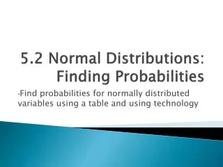
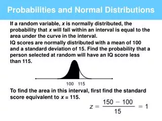
Normal Distribution Also known as the Gaussian distribution, after Karl Gauss. This is the expected distribution when many randomly distributed factors add together. It is found in distributions of body height/weight, chemical concentrations in soil/air/water, and many other situations. Note the symmetrical bell-shaped curve Number of observations Size of value Mean and median about the same
Carl Friedrich Gauss30/4/1777 – 23/2/1855 The Gaussian distribution was one of the many deeply significant mathematical discoveries made by Carl Gauss, who was probably the greatest mathematician in history. At the age of 7, when he started school, he was asked (by an exasperated tutor who wanted to put this little upshot in his place) to add up the numbers from 1+2+3…+99+100. Little Carl promptly and contemptuously write down 5050 on his slate and threw it onto the teacher’s desk! How we think he did it: 1 + 100 = 101 2 + 99 = 101 3 + 98 = 101 Etc There are 50 such pairs: 50*101 = 5050
You only need 2 numbers to define a Normal curve:The mean μThe standard deviation σ Any observation in a dataset can be re-coded in terms of how many standard deviations away from the mean it lies σ μ
A powerful universal principal: • The Normal distribution is immensely useful because it is universal: The same shape describes human height, hardness of stones, strength of winds… • The way to convert any arbitrary set of data into the universal distribution is to recode as follows: • Convert each observation into a number telling you how many s.d.s it is away from the mean. • This is called a Z score (I don’t know why): • Zi = (Xi- μ)/σ
And the point of this? • Is that you can look up Z scores in tables, confident in the knowledge that: • C. 66% of the points will lie between Z=-1.0 and Z=1.0 (ie within 1 sd of the mean) • C. 95% of the points lie within +- 2sd of the mean • 99.9% of points are within+- 3sd of mean
We’ll try this out! • Measure the length of your left index finger, in mm. • I’ll enter a subset into the PC, and we’ll see whether a Gaussian curve emerges. • Given the mean + sd, you work out your own Z score!
You should know: That the area under the standard normal curve Corresponds to probability, specifically the probability Of finding an observation less than a given Z value. The total area under the curve, from infinity to – infinity = 1.0 You don’t need to know: Equation of curve is: Y = 1/(2π) ½ exp(-½Z*Z)
Z = 0, area = above Z = 0.5, ie half the curve lies below the mean Z = 1.0, area = above Z =0.1587, ie about 85% data lies below (mean + 1 sd)
Applied example: • A factory making widgets can only sell those whose length is between 98 and 101 mm diameter. • The machine makes widgets with a mean of 100mm and an sd of 0.7mm. • What % of widgets are rejected as unsaleable due to size? Convert data into Z scores: 98 (98-100)/0.7 = -2.85 101 (101-100)/0.7 = 1.42
Area above Z = 1.42. = 0.159 Area below Z = -2.8 = 0.003 Acceptable area (purple) = 1- (0.159+ 0.003) = 0.838 Upper tail of distribution, area = 0.1587 Lower tail of distribution area = 0.003
Often real data don’t follow the Normal curve but are skewed – here organic content in heath soils Try log-transforming the data. Here the same data after calculating log of the numbers – not perfect, but clearly more symmetrical
How to decide about normality? • Inspect histogram + fitted normal curve. • Inspect a cumulative “P-P curve” with predicted normal distribution • Run the Kolgomorov-Smirnov test
The Kolgomorov-Smirnov test examines whether data can be assumed to come from a chosen distribution – here the normal. LogLOI may or may not be normal, but the test tells us that its deviations from normality would occur 7 times in 10 in randomly chosen normal data LOI is almost certainly NOT normally distributed