Probabilities and Expected Values
Probabilities and Expected Values. Normal Distribution, Statistical Inference, Central Limit Theorem. The Probability of any Set of Events. 1 =< Probability >= 0. A B C. Probability of A or B or C happening = 1

Probabilities and Expected Values
E N D
Presentation Transcript
Normal Distribution, Statistical Inference, Central Limit Theorem
The Probability of any Set of Events 1 =< Probability >= 0 A B C Probability of A or B or C happening = 1 (This is true as long as events A, B and C are exhaustive and mutually exclusive)
Probability Probability of drawing a blue balloon: 4/12 = 1/3 Probability of drawing a red balloon: 3/12 = 1/4 Probability of drawing a blue balloon: 5/12
Expected Value If we did this over and over, we expect to get blue balloons 1/3 of the time If we did this over and over, we expect to get red balloons 1/4 of the time If we did this over and over, we expect to get blue balloons 5/12 of the time
Probability: Sampling from Population Inferential Statistics: Making Claims about a Population
What are we interested in knowing about? Point estimates (means, correlations, slopes…) How confident are we about those estimates?
Question: What is the likelihood that this sample comes from a population with a point estimate of ____. Answer depends on: Variation around that estimate Number of cases in the sample
Population Low Support for Democracy Medium Support for Democracy High Support for Democracy
For a sample estimate to approach the population estimate, the sample must be random. This means that every case has an equal probability of being selected.
Support for Democracy Medium 2 High 3 High 3 Low 1 Low 1 Medium 2 Low 1 Low 1 Medium 2 High 3 High 3 High 3 Sample Mean = 2.08 Median? Mode?
6 5 4 Frequency Normal curve 3 2 1 Std. Dev = .90 Mean = 2.08 N = 12.00 0 1.00 1.50 2.00 2.50 3.00 Support for Democracy Histogram: A Probability Distribution
Probability of selecting a person with low support for democracy: 4/12 = 1/3 Probability of selecting a person with medium support for democracy = 1/4 Probability of selecting a person with medium support for democracy = 5/12 = .42
Conditional Probabilities: Relationships
What is the probability of having high support for democracy if you have a low income? What is the probability of having high support for democracy if you have a medium income? What is the probability of having high support for democracy if you have a high income?
Normal Distribution, Statistical Inference, Central Limit Theorem
The Normal Distribution • Symmetric • Continuous = prob of any one point = zero, because the area of a line is zero – we always compute probabilities of lying between some designated x and y • All have same general shape • Cases more concentrated in the middle than in the tails • Shape determined by: mean and standard deviation • The area under the curve is 1 • The probability of any event under the curve is determined by the height of the curve at that place Number of cases = y axis Value of the variable = x axis
Approximately 68 percent of the area under a normal curve lies between the values of the mean and the standard deviation + and – the mean. • Approximately 95% of the area lies between 2 standard deviations + and – the mean. • Approximately 99.7% lies between 3 standard deviations + and – the mean.
The Standard Normal Distribution Same as a normal distribution, but the standard deviation is 1 and the mean is 0 0
Any normal distribution can be turned into a standard normal with a linear transformation: 1) Subtract the mean from every observation 2) Divide by the standard deviation This is called a z-score.
The Central Limit Theorem Given a population with ANY distribution: Taking random samples of size n from that distribution The sample means will be (approximately) normally distributed.
Sampling Distribution Illustration http://www.ruf.rice.edu/%7Elane/stat_sim/sampling_dist/index.html
Why do we care about the Normal Distribution? 1) Many of the political phenomena that we study are distributed normally. For example, Ideology – there are lots of people in the middle and not as many people on the tails 2) The normal distribution has some cool properties, like being able to easily compute percentiles.
Assume grades on a test are normally distributed mean of 80 standard deviation of 5 What is the percentile rank of a person who received a score of 70 on the test?
To take another example, what is the percentile rank of a person receiving a score of 90 on the test?
If a test is normally distributed with a mean of 60 and a standard deviation of 10, what proportion of the scores are above 85? A z table can be used to calculate that .9938 of the scores are less than or equal to a score 2.5 standard deviations above the mean. It follows that only 1-.9938 = .0062 of the scores are above a score 2.5 standard deviations above the mean. Therefore, only .0062 of the scores are above 85. Given the sample, what is the probability of selecting out a test grade higher than 85?
Properties of Estimators Remember that Ordinary Least Squares minimizes the squared errors from the line.
Residuals of OLS analysis (errors of the slope) have a mean of zero, by definition – they have been computed by their minimization. We also assume that they are distributed normally. Therefore they are distributed along a standard normal distribution, mean of zero. (The standard deviation is not necessarily 1, but it is assumed to be constant across all values of x). Foreshadowing: if this assumption does not hold, you cannot use OLS.
The Null Hypothesis What is the question that we ask with statistics? Answer: How likely is it that the relationship is zero? The null hypothesis is that the relationship is zero. We are trying to reject the null hypothesis.
We have a point estimate – we call it a slope, but we cannot be sure about that point because we do not know anything about the population. So, we know that there is error in our estimate. So, neither the upper bound and lower bound of our estimate can contain zero.
Generally, we want to be at least 95% confident that our estimate does not include zero. 0 So, to be 95% confident that the true estimate does not contain zero, then the estimate must be two standard deviations from the mean of the standard normal curve, which is zero.
If a certain interval is a 95% confidence interval, then we can say that if we repeated the procedure of drawing random samples and computing confidence intervals over and over again, 95% of those confidence intervals include the true value from the population. This is not to say that we are 98% confident that the true value lies between the upper and lower bound. Instead, I am 98% confident that a Confidence interval “covers” the true value from the population, based not on this single CI from this single test, but rather as a result of what would happen were I to repeat the process of drawing samples and doing this test over and over again.
Effect of Index of Signals on the Number of Cases on the U.S Supreme Court Agenda, 1953-1995 8 7 6 4.62 5 3.85 Upper bound of the 95% confidence interval Estimate Lower bound of the 95% confidence interval 4 3 2.11 2 1.27 1.19 1.34 1 0 -1 1 2 3 4 5 6 -2 Lag Year Note: Note: Estimates are Ordinary Least Square unstandardized regression coefficients and confidence intervals are computed using panel corrected standard errors, calculated according to Beck and Katz (1995). Controls in this analysis include policy area dummy variables, Burger and Rehnquist Court dummies, the legislative agenda, ideological output of the Supreme Court, and absolute value change of median voter. The dependent variable is the number of cases on the Supreme Court’s agenda, across 11 policy areas from 1953-1995. The independent variable presented here is an index of salient cases, as measured by Epstein and Segal (1996), declarations of constitutionality, the number of lower court reversals and formal alterations of precedent.
12 10 8 6.95 6.48 6 Upper bound of the 95% confidence interval Estimate Lower bound of the 95% confidence interval 4.61 3.92 4 2.93 2.37 2 0 -2 1 2 3 4 5 6 R2 = .83 n = 232 Lag Year The Effect of Supreme Court Signals on Amicus Briefs at Courts of Appeals
The Effect of the Legislative Agenda on the Supreme Court Agenda 10 8 6 4 2 0 -2 -4 -6 -8 -10 -12 R2 = .63 n = 407 1 2 3 4 5 6 Lag Year Upper bound 95% Confidence Interval Point Estimate - slope Lower bound 95% Confidence Interval
1 2 3 4 5 6 The Effect of the Legislative Agenda on the Appeals Courts’ Agendas Lag Year 25 20 15 10 5 0 -5 -10 -15 -20 R2 = .64 n = 240 Upper bound 95% Confidence Interval Point Estimate - slope Lower bound 95% Confidence Interval