Download

1 / 34
350 likes | 494 Vues
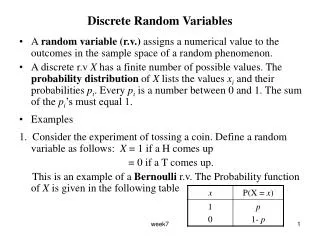
Expected values of discrete Random Variables. Definition of Discrete RV (Review). The function that maps S into S X in R and which is denoted by X (.) is called a random variable .

E N D
Definition of Discrete RV (Review) • The function that maps S into SX in R and which is denoted by X(.) is called a random variable. • The name random variable is a poor one in that the function X(.) is not random but a known one and usually one of our own choosing. • Example: In phase-shift keyed (PSK) digital system a ”0” or “1” is communicated to a receiver by sending • A 1 or a 0 occurs with equal probability so we model the choice of a bit as a fair coin tossing experiment. random variable
Last lecture overview: Example Servicing Customers • A supermarket has one express lane open from 5 to 6PM on weekdays. • No more than 10 items are allowed, thus average time is 1 min. • The supermarket wants that no more that one person waiting in line 95% of the time. • How many lanes should be opened?
Example: Servicing Customers • Since the processing time is 1 min, there can be at most two arrivals in each time slot of 1 min length. (One is serviced and the other is waiting for a min). • Assuming no two arrivals per second is possible we have a sequence of independent Bernoulli trials • 0 – no arrivals • 1 - arrival
Example: Servicing Customers • Observing the total arrivals, the average is 70 arrivals per min or 70 per 3600 seconds. Thus probability of arrival is p= 70 / 3600 = 0.0194. • We have the Binomial PMF, with p = 0.0194 and M = 60 seconds. • Approximating it with Poisson PMF, the probability of k arrivals in 60 seconds is • Where is expected number of customers arriving in the 1 minute interval.
Example: Servicing Customers • There should be at most 2 customers arriving 95% of the time. • Substituting Poisson PMF • Hence, the probability of 2 or fewer customers arriving at the express lane is not grater than 0.95. • Adding one more lane, we have 70/2=35 customers per minute. Therefore .
Example: Servicing Customers • Since the arrivals are modeled as independent Bernoulli trials, so that
Probability Mass Functions • PMF is a complete description of a discrete random variable. • It allows to determine probabilities of any event. Estimated PMF 9.76 • We might be interested in a rainfall between 8 and 12 inches to grow a particular crop. Is this adequate or should the probability be higher?
Determining Averages from the PMF • Rather it might be more useful to know the average rainfall, since it is close to the requirement of an adequate amount of rainfall. • Two methods to estimate average
Determining Averages from the PMF • Example: A barrel is filled with equal number of US dollar bills $1,5,10,20. • A person playing the game gets to choose a bill from the barrel, but must do so blindfolded. • He pays 10$ to play the game, which consists of a single draw with replacement from the barrel. He wins that amount of money. Will he make a profit by playing this game? The average of winning per play
Determining Averages from the PMF The number of times a player wins k dollars N1 = 13, N2= 13, N10 = 10, N20 = 14 If he were to play the game a large number of times, then N∞ we would have Nk/N pX[k]. pX[k] is PMF of choosing a bill with k$. On average he will lose $1 per play Proportion of bills
Determining Averages from the PMF • The expected value is also called the expectation of X,the average of X, and the mean of X. • The expected value of a discrete RV X is defined as For all nonzero pX[xi]. • The expected value may be interpreted as the best prediction of the outcome of a random experiment for a single trial. • The expected value is analogous to the center of mass of a system of linearly arranged masses. Expected value
Expected values of Important Random Variables. • Bernoulli: If X ~ Ber(p), then the expected value is • BinomialX: If X ~ bin(M, p), then the expected value is SettingM/ = M – 1, k/ = k -1, this becomes
Expected values of Important Random Variables. • Geometric: if X ~ geom(p), the expected value is • Let’s modify the summand to be a PMF by letting q =1 – pand then differentiating the expression • Since 0 < q < 1 we have Σk=1..∞qk = q/(1 - q) • If p = 1/10, then on average it takes 10 trials for a success.
Expected values of Important Random Variables. • Poisson: If X ~ Pois(p), then it can be shown that E[X] = λ. • This result is consistent with the Poisson approximation to the binomial PMF since the approximation constrains Mp to λ. Not all PMFs have expected values. • Discrete RVs with a finite number of values always have expected values. • Discrete RVs with countably infinite number of values may not have an expected value. • Consider the PMF • Attempting to find the expected value produces It is valid PMF since it can be show to sum to one
Expected values of Important RV • It is possible for a sum to produce different results depending upon the order in which the terms are added up. • To avoid these difficulties, we require the sum to be absolutely summable.
Properties of the expected value • It is located at the “center” of the PMF if the PMF is symmetric about some point. • It does not generally indicate the most probable value of RV. • More than one PMF may have the same expected value.
Expected Value for a Function of RV • The expected value may easily be found for a function of RVX if pX[xi] is known. • If the function of interest is Y = g(X), then by the definition of expected value • or in much convenient form
Expected Value for a Function of RV • A linear function • If g(x) = aX + b, where aand b are constants, then • If we set a = 1, then E[X + b] = E[X] + b. This allows us to set the expected value of a RV to any desired value by adding the appropriate constant to X. • An extension produces For any constants a1 and a2 and any two functions g1 and g2. Thus, expectation operator E is linear.
Expected Value for a Function of RV • A nonlinear function: Assume that X has a uniform PMF given by Determine E[Y] for Y = g(X) = X2. It is not true that The expectation operator does not commute for nonlinear functions.
Variance and Moments of a RV • The variability or variance is another important information about RV’s behavior and it given by • Example: a uniform discrete RV is given whose PMF is • mean is zero but variability of the outcomes becomes large as M increases. M = 2 M = 10
Variance and Moments of a RV It can be shown that assume zero Which yields Clearly, variance increases with M M = 2 M = 10
Variance of Bernoulli RV • If X ~ Ber(p), then since E[X] = p, we have The variance is minimized and equals zero if p = 0 or p = 1.It is maximized for p =1/2. Why? • The best predictor bopt = E[X]. • We wish to point out the minimum MSE. How well we can predict the outcome depends on the variance of RV.
An alternative expression for the variance • Applying properties of expectation operator we have • Hence • In the case where E[X] = 0, we have the simple result that var(X) = E[X2]
Properties of the variance • Property 1. Alternative expression for variance • Property 2. Variance for RV modified by a constant • For c a constant • The expectations E[X] and E[X2] are called the first and second moments of X. Generally, nth moment is defined as E[Xn] and exists if E[|X|n]. • Central moments defined as E[(X – E[X])n]. For n = 2 we have the usual definition of the variance. • Variance is a nonlinear operator
Real-world example: Data compression • Data consists of a sequence of the letters A, B, C, D. • Consider a typical sequence of 50 letters • AAAAAAAAAAABAAAAAAAAAAAAA • AAAAAACABADAABAAABAAAAAAD • To encode these letters for storage we could use the two-bit code • A 00 • B 01 • C 10 • D 11 • Which would then require a storage of 2 bits per letter for a total storage of 100 bits. • The above sequence is characterized by a much larger probability of observing “A” as opposed to the other letters. • 43 A’s, 4 B’s, 1 C, and 2D’s.
Real-world example: Data compression • It makes sense then to attempt a reduction in storage by assigning shorter code words to the letters that occur more often, in this case, to the “A”. • A 0 • B 10 • C 110 • D -> 111 • Using this code, would require 1 43 + 2 4 + 3 1 + 32 = 60 bits or 1.2 bits per letter. Huffman code • To determine storage savings we need to determine the average length of the code word per letter. First we define a discrete RV that measures the length of the code word.
Real-world example: Data compression • The probability used to generate the sequence of letters are P[A] = 7/8, P[B] = 1/16, P[C] = 1/32, P[D] = 1/32. The PMF is • The average code length is give by • This result in a compression ratio of 2 : 1,1875 = 1.68 or we require about 40% less storage. bits per letter
Real-world example: Data compression • The average code word length per letter can be reduced even further. However it requires more complexity in coding. • A fundamental theorem due to Shannon, says that the average code word length per letter can be no less than • The quantity is termed the entropy of the source. In addition, he showed that a code exist that can attain, this minimum average code length. • Hence, the potential compression ratio is 2:0.7311 = 2.73 for a bout 63% reduction. If P[si] = ¼, bits per letter bits per letter No compression is possible
Problems 1) 2) 3) 4) A discrete RV X has the PMF pX[k] = 1/5 for k =0,1,2,3,4. If Y = sin[(π/2)X] find E[Y] using Which way is easier?
Estimate Means and Variances • Define xi and pX using given PMF • Estimate and plot means and variance
H/W problems 1) 2) (a) (b) (c)