Expected Values
Expected Values. Once we have defined a random variable for our experiment, we can statistically analyze the outcomes of the experiment.

Expected Values
E N D
Presentation Transcript
Expected Values • Once we have defined a random variable for our experiment, we can statistically analyze the outcomes of the experiment. • For example, we can ask: What is the average value (called the expected value) of a random variable when the experiment is carried out a large number of times? • Can we just calculate the arithmetic mean across all possible values of the random variable? Applied Discrete Mathematics Week 10: Advanced Counting
Expected Values • No, we cannot, since it is possible that some outcomes are more likely than others. • For example, assume the possible outcomes of an experiment are 1 and 2 with probabilities of 0.1 and 0.9, respectively. • Is the average value 1.5? • No, since 2 is much more likely to occur than 1, the average must be larger than 1.5. Applied Discrete Mathematics Week 10: Advanced Counting
Expected Values • Instead, we have to calculate the weighted sum of all possible outcomes, that is, each value of the random variable has to be multiplied with its probability before being added to the sum. • In our example, the average value is given by0.11 + 0.92 = 0.1 + 1.8 = 1.9. • Definition: The expected value (or expectation) of the random variable X(s) on the sample space S is equal to: • E(X) = sSp(s)X(s). Applied Discrete Mathematics Week 10: Advanced Counting
Expected Values • Example: Let X be the random variable equal to the sum of the numbers that appear when a pair of dice is rolled. • There are 36 outcomes (= pairs of numbers from 1 to 6). • The range of X is {2, 3, 4, 5, 6, 7, 8, 9, 10, 11, 12}. • Are the 36 outcomes equally likely? • Yes, if the dice are not biased. • Are the 11 values of X equally likely to occur? • No, the probabilities vary across values. Applied Discrete Mathematics Week 10: Advanced Counting
Expected Values 1/36 P(X = 3) = 2/36 = 1/18 P(X = 4) = 3/36 = 1/12 • P(X = 2) = P(X = 5) = 4/36 = 1/9 P(X = 6) = 5/36 P(X = 7) = 6/36 = 1/6 P(X = 8) = 5/36 P(X = 9) = 4/36 = 1/9 P(X = 10) = 3/36 = 1/12 P(X = 11) = 2/36 = 1/18 P(X = 12) = 1/36 Applied Discrete Mathematics Week 10: Advanced Counting
Expected Values • E(X) = 2(1/36) + 3(1/18) + 4(1/12) + 5(1/9) + 6(5/36) + 7(1/6) + 8(5/36) + 9(1/9) + 10(1/12) + 11(1/18) + 12(1/36) • E(X) = 7 • This means that if we roll the dice many times, sum all the numbers that appear and divide the sum by the number of trials, we expect to find a value of 7. Applied Discrete Mathematics Week 10: Advanced Counting
Expected Values • Theorem: • If X and Y are random variables on a sample space S, then E(X + Y) = E(X) + E(Y). • Furthermore, if Xi, i = 1, 2, …, n with a positive integer n, are random variables on S, thenE(X1 + X2 + … + Xn) = E(X1) + E(X2) + … + E(Xn). • Moreover, if a and b are real numbers, then E(aX + b) = aE(X) + b. • Note the typo in the textbook! Applied Discrete Mathematics Week 10: Advanced Counting
Expected Values • Knowing this theorem, we could now solve the previous example much more easily: • Let X1 and X2 be the numbers appearing on the first and the second die, respectively. • For each die, there is an equal probability for each of the six numbers to appear. Therefore, E(X1) = E(X2) = (1 + 2 + 3 + 4 + 5 + 6)/6 = 7/2. • We now know that E(X1 + X2) = E(X1) + E(X2) = 7. Applied Discrete Mathematics Week 10: Advanced Counting
Expected Values • We can use our knowledge about expected values to compute the average-case complexity of an algorithm. • Let the sample space be the set of all possible inputs a1, a2, …, an, and the random variable X assign to each aj the number of operations that the algorithm executes for that input. • For each input aj, the probability that this input occurs is given by p(aj). • The algorithm’s average-case complexity then is: • E(X) = j=1,…,np(aj)X(aj) Applied Discrete Mathematics Week 10: Advanced Counting
Expected Values • However, in order to conduct such an average-case analysis, you would need to find out: • the number of steps that the algorithms takes for any (!) possible input, and • the probability for each of these inputs to occur. • For most algorithms, this would be a highly complex task, so we will stick with the worst-case analysis. • In the textbook (page 283 in the 4th Edition, page 384 in the 5th Edition , page 431 in the 6thEdition , page 482 in the 7thEdition), an average-case analysis of the linear search algorithm is shown. Applied Discrete Mathematics Week 10: Advanced Counting
Independent Random Variables • Definition: The random variables X and Y on a sample space S are independent if • p(X(s) = r1 Y(s) = r2) = p(X(s) = r1) p(Y(s) = r2). • In other words, X and Y are independent if the probability that X(s) = r1 Y(s) = r2 equals the product of the probability that X(s) = r1 and the probability that Y(s) = r2 for all real numbers r1 and r2. Applied Discrete Mathematics Week 10: Advanced Counting
Independent Random Variables • Example: Are the random variables X1 and X2 from the “pair of dice” example independent? • Solution: • p(X1 = i) = 1/6 • p(X2 = j) = 1/6 • p(X1 = i X2 = j) = 1/36 • Since p(X1 = i X2 = j) = p(X1 = i)p(X2 = j) ,the random variables X1 and X2 are independent. Applied Discrete Mathematics Week 10: Advanced Counting
Independent Random Variables • Theorem: If X and Y are independent random variables on a sample space S, thenE(XY) = E(X)E(Y). • Note: • E(X + Y) = E(X) + E(Y) is true for any X and Y, but • E(XY) = E(X)E(Y) needs X and Y to be independent. • How come? Applied Discrete Mathematics Week 10: Advanced Counting
Independent Random Variables • Example: Let X and Y be random variables on some sample space, and each of them assumes the values 1 and 3 with equal probability. • Then E(X) = E(Y) = 2 • If X and Y are independent, we have: • E(X + Y) = 1/4·(1 + 1) + 1/4·(1 + 3) + 1/4·(3 + 1) + 1/4·(3 + 3) = 4 = E(X) + E(Y) • E(XY) = 1/4·(1·1) + 1/4·(1·3) + 1/4·(3·1) + 1/4·(3·3) = 4 = E(X)·E(Y) Applied Discrete Mathematics Week 10: Advanced Counting
Independent Random Variables • Let us now assume that X and Y are correlated in such a way that Y = 1 whenever X = 1, and Y = 3 whenever X = 3. • E(X + Y) = 1/2·(1 + 1) + 1/2·(3 + 3) = 4 = E(X) + E(Y) • E(XY) = 1/2·(1·1) + 1/2·(3·3) = 5 E(X)·E(Y) Applied Discrete Mathematics Week 10: Advanced Counting
Variance • The expected value of a random variable is an important parameter for the description of a random distribution. • It does not tell us, however, anything about how widely distributed the values are. • This can be described by the variance of a random distribution. Applied Discrete Mathematics Week 10: Advanced Counting
Variance • Definition: Let X be a random variable on a sample space S. The variance of X, denoted by V(X), is • V(X) = sS(X(s) – E(X))2p(s). • The standard deviation of X, denoted by (X), is defined to be the square root of V(X). Applied Discrete Mathematics Week 10: Advanced Counting
Variance • Useful rules: • If X is a random variable on a sample space S, thenV(X) = E(X2) – E(X)2. • If X and Y are two independent random variables on a sample space S, then V(X + Y) = V(X) + V(Y). • Furthermore, if Xi, i = 1, 2, …, n, with a positive integer n, are pairwise independent random variables on S, then V(X1 + X2 + … + Xn) = V(X1) + V(X2) + … + V(Xn). • Proofs in the textbook on pages 280 and 281 (4th Edition), pages 389 and 390 (5th Edition), pages 436 and 437 (6thEdition), and pages 488-490 (7thEdition). Applied Discrete Mathematics Week 10: Advanced Counting