Instrumentation

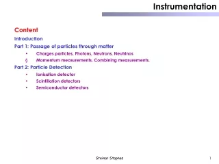
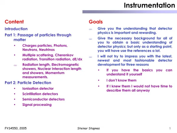
Instrumentation • Content Introduction Part 1: Passage of particles through matter • Charges particles, Photons, Neutrons, Neutrinos • Multiple scattering, Cherenkov radiation, Transition radiation, dE/dx • Radiation length, Electromagnetic showers, Nuclear Interaction length and showers, Momentum measurements. Part 2: Particle Detection • Ionisation detector • Scintillation detectors • Semiconductor detectors • Signal processing • Goals • Give you the understanding that detector physics is important and rewarding. • Give the necessary background for all of you to obtain a basic understanding of detector physics; but only as a starting point, you will have use the references a lot. • I will not try to impress you with the latest, newest and most fashionable detector development for three reasons • If you have the basics you can understand it yourself • I don’t know them • If I knew them I would not have time to describe them all anyway Steinar Stapnes

Instrumentation • Experimental Particle Physics Accelerators • Luminosity, energy, quantum numbers Detectors • Efficiency, speed, granularity, resolution Trigger/DAQ • Efficiency, compression, through-put, physics models Offline analysis • Signal and background, physics models. The primary factors for a successful experiment are the accelerator and detector/trigger system, and losses there are not recoverable. New and improved detectors are therefore extremely important for our field. Steinar Stapnes

Instrumentation These lectures are mainly based on seven books/documents : (1) W.R.Leo; Techniques for Nuclear and Particle Physics Experiments. Springer-Verlag, ISBN-0-387-57280-5; Chapters 2,6,7,10. (2 and 3) D.E.Groom et al.,Review of Particle Physics; section: Experimental Methods and Colliders; see http://pdg.web.cern.ch/pdg/ Section 27: Passage or particles through matter Chapter 28 : Particle Detectors. (4) Particle Detectors; CERN summer student lectures 2002 by C.Joram, CERN. These lectures can be found on the WEB via the CERN pages, also video-taped. Also newer summer students lecture series can be useful. • Instrumentation; lectures at the CERN CLAF shool of Physics 2001 by O.Ullaland, CERN. The proceeding is available via CERN. • K.Kleinknecht; Detectors for particle radiation. Cambridge University Press, ISBN 0-521-64854-8. • G.F.Knoll; Radiation Detection and Measurement. John Wiley & Sons, ISBN 0-471-07338-5 • In several cases I have included pictures from (4) and (5) and text directly in my slides (indicated in my slides when done). • I would recommend all those of you needing more information to look at these sources of wisdom, and the references. Steinar Stapnes

Instrumentation Concentrate on electromagnetic forces since a combination of their strength and reach make them the primary responsible for energy loss in matter. For neutrons, hadrons generally and neutrinos other effects obviously enter. Steinar Stapnes

Strength versus distance Steinar Stapnes

Heavy charged particles Heavy charged particles transfer energy mostly to the atomic electrons, ionising them. We will later come back to not so heavy particles, in particular electrons/positrons. Usually the Bethe Bloch formally is used to describe this - and most of features of the Bethe Bloch formula can be understood from a very simple model : 1) Let us look at energy transfer to a single electron from heavy charged particle passing at a distance b 2) Let us multiply with the number of electrons passed 3) Let us integrate over all reasonable distances b electron,me b ze,v Steinar Stapnes

The impulse transferred to the electron will be : • The integral is solved by using Gauss’ law over an infinite cylinder (see fig) : • The energy transfer is then : • The transfer to a volume dV where the electron density is Ne is therefore : • The energy loss per unit length is given by : • bmin is not zero but can be determined by the maxium energy transferred in a head-on collision • bmax is given by that we require the perturbation to be short compared to the period ( 1/v) of the electron. • Finally we end up with the following which should be compared to Bethe Bloch formula below : • Note : • dx in Bethe Bloch includes density (g cm-2) Steinar Stapnes

Bethe Bloch parametrizes over momentum transfers using I (the ionisation potential) and Tmax (the maximum transferred in a single collision) : The correction  describe the effect that the electric field of the particle tends to polarize the atoms along it part, hence protecting electrons far away (this leads to a reduction/plateau at high energies). The curve has minimum at =0.96 (=3.5) and increases slightly for higher energies; for most practical purposed one can say the curve depends only on  (in a given material). Below the Minimum Ionising point the curve follows -5/3. At low energies other models are useful (as shown in figure). The radiative losses at high energy we will discuss later (in connection with electrons where they are much more significant at lower energies). Steinar Stapnes

Bethe Bloch basics A more complete description of Bethe Bloch and also Cherenkov radiation and Transition Radiation – starting from the electromagnetic interaction of a particle with the electrons and considering the energy of the photon exchanged – can be found in ref. 6 (Kleinknecht). Depending on the energy of the photon one can create Cherenkov radiation (depends on velocity of particle wrt speed of light in the medium), ionize (Bethe Bloch energy loss when integrating from the ionisation energy to maximum as on previous page), or create Transition Radiation at the border of two absorption layers with different materials. See also references to articles of Allison and Cobb in the book. Steinar Stapnes

Processes as function of photon energy Steinar Stapnes

Heavy charges particles Steinar Stapnes

Heavy charged particles The ionisation potential (not easy to calculate) : Steinar Stapnes

Heavy charged particles Since particles with different masses have different momenta for same  Steinar Stapnes

Heavy charged particles While Bethe Bloch describes the average energy deposition, the probability distribution is described by a Landau distribution . Other functions are ofter used : Vavilov, Bichsel etc. In general these a skewed distributions tending towards a Gaussian when the energy loss becomes large (thick absorbers). One can use the ratio between energy loss in the absorber under study and Tmax from Bethe Bloch to characterize thickness. Steinar Stapnes

Electrons and Positrons Electrons/positrons; modify Bethe Bloch to take into account that incoming particle has same mass as the atomic electrons Bremsstrahlung in the electrical field of a charge Z comes in addition :  goes as 1/m2 e e  The critical energy is defined as the point where the ionisation loss is equal the bremsstrahlung loss. Steinar Stapnes

Electrons and Positrons The differential cross section for Bremsstrahlung (v : photon frequency) in the electric field of a nucleus with atomic number Z is given by (approximately) : The bremsstrahlung loss is therefore : where the linear dependence is shown. The  function depends on the material (mostly); and for example the atomic number as shown. N is atom density of the material (atoms/cm3). Bremsstrahlung in the field of the atomic electrons must be added (giving Z2+Z). A radiation length is defined as thickness of material where an electron will reduce it energy by a factor 1/e; which corresponds to 1/N as shown on the right (usually called 0). e  Steinar Stapnes

Electrons and Positrons Steinar Stapnes

Electrons and Positrons Radiation length parametrisation : A formula which is good to 2.5% (except for helium) : A few more real numbers (in cm) : air = 30000cm, scintillators = 40cm, Si = 9cm, Pb = 0.56cm, Fe = 1.76 cm. Steinar Stapnes

Photons • Photons important for many reasons : • Primary photons • Created in bremsstrahlung • Created in detectors (de-excitations) • Used in medical applications, isotopes • They react in matter by transferring all (or most) of their energy to electrons and disappearing. So a beam of photons do not lose energy gradually; it is attenuated in intensity (only partly true due to Compton scattering). Steinar Stapnes

Photons Three processes : Photoelectric effect (Z5); absorption of a photon by an atom ejecting an electron. The cross-section shows the typical shell structures in an atom. Compton scattering (Z); scattering of a photon again a free electron (Klein Nishina formula). This process has well defined kinematic constraints (giving the so called Compton Edge for the energy transfer to the electron etc) and for energies above a few MeV 90% of the energy is transferred (in most cases). Pair-production (Z2+Z); essentially bremsstrahlung again with the same machinery as used earlier; threshold at 2 me = 1.022 MeV. Dominates at a high energy. Plots from C.Joram Steinar Stapnes

Photons Considering only the dominating effect at high energy, the pair production cross-section, one can calculate the mean free path of a photon based on this process alone and finds : Ph.El. Pair Prod. Compton Steinar Stapnes

Electromagnetic calorimeters From C.Joram Considering only Bremsstrahlung and Pair Production with one splitting per radiation length (either Brems or Pair) we can extract a good model for EM showers. Steinar Stapnes

Electromagnetic calorimeters More : Text from C.Joram Text from C.Joram Steinar Stapnes

Electromagnetic calorimeters The total track length : Intrinsic resolution : Text from C.Joram Steinar Stapnes

Electromagnetic calorimeters From Leo Text from C.Joram Steinar Stapnes

CERN-Claf, O.Ullaland Sampling Calorimeter A fraction of the total energy is sampled in the active detector Particle absorption Shower sampling is separated. Active detector : Scintillators Ionization chambers Wire chambers Silicon E N at 1 GeV Steinar Stapnes

CERN-Claf, O.Ullaland Homogeneous Calorimeter The total detector is the active detector. N  E (E)  Limited by photon statistics E at 1 GeV N Crystal Ball NaI(Tl) E. Longo, Calorimetry with Crystals, submitted to World Scientific, 1999 CLEO ll CsI(TI) Resolution .01 BGO 10 Steinar Stapnes Energy (GeV)

Neutrons Steinar Stapnes Text from C.Joram

Absorption length and Hadronic showers Text from C.Joram Define hadronic absorption and interaction length by the mean free path (as we could have done for 0) using the inelastic or total cross-section for a high energy hadrons (above 1 GeV the cross-sections vary little for different hadrons or energy). Steinar Stapnes

Text from C.Joram Steinar Stapnes

Neutrinos Steinar Stapnes Text from C.Joram

Summary of reactions with matter • The basic physics has been described : • Mostly electromagnetic (Bethe Bloch, Bremsstrahlung, Photo-electric effect, Compton scattering and Pair production) for charged particles and photons; introduce radiation length and EM showers • Additional strong interactions for hadrons; hadronic absorption/interaction length and hadronic showers • Neutrinos weakly interacting with matter Steinar Stapnes

Next steps How do we use that fact that we now know how most particles ( i.e all particles that live long enough to reach a detector; e,,p,,k,n,photons, neutrinos,etc) react with matter ? Q: What is a detector supposed to measure ? A1 : All important parameters of the particles produced in an experiment; p, E, v, charge, lifetime, identification, etc With high efficiency and over the full solid angle of course. A2 : Keeping in mind that secondary vertices and combinatorial analysis provide information about c,b-quarks, ’s, converted photons, neutrinos, etc • Next steps; look at some specific measurements where “special effects” or clever detector configuration is used: • Cherenkov and Transitions radiation important in detector systems since the effects can be used for particle ID and tracking, even though energy loss is small • This naturally leads to particle ID with various methods • dE/dx, Cherenkov, TRT, EM/HAD, p/E • Look at magnetic systems and multiple scattering • Secondary vertices and lifetime Steinar Stapnes

Cherenkov 5 4 3 2 eV A particle with velocity =v/c in a medium with refractive index n may emit light along a conical wave front if the speed is greater than speed of light in this medium : c/n CERN-Claf, O.Ullaland The angle of emission is given by and the number of photons by Steinar Stapnes

Cherenkov CERN-Claf, O.Ullaland Threshold Cherenkov Counter, chose suitable medium (n) Cherenkov gas Particle with charge q velocity b Spherical mirror Flat mirror Photon detector To get a better particle identification, use more than one radiator. Steinar Stapnes

Cherenkov Detector CERN-Claf, O.Ullaland Focusing Mirror Cherenkov media e- e+ Proportional Chamber g g g Quartz Plate e e e E Photon to Electron conversion gap Steinar Stapnes

Cherenkov n = 1.28 C6F14 liquid p/K p/K/p K/p n = 1.0018 C5F12 gas p/h p/K/p K/p CERN-Claf, O.Ullaland Particle Identification in DELPHI at LEP I and LEP II • 0.7  p  45 GeV/c • 15°  q  165° Liquid RICH Gas RICH 2 radiators + 1 photodetector Steinar Stapnes

Cherenkov CERN-Claf, O.Ullaland Liquid RICH Cherenkov angle (mrad) Gas RICH p (GeV) From data p from L K from F D* p from Ko Steinar Stapnes

Transition Radiation Electromagnetic radiation is emitted when a charged particle transverses a medium with discontinuous refractive index, as the boundary between vacuum and a dielectric layer. B.Dolgosheim (NIM A 326 (1993) 434) for details. Energy per boundary : Only high energy e+- will emit TR, electron ID. Plastic radiators An exact calculation of Transition Radiation is complicated (J. D. Jackson) and he continues: A charged particle in uniform motion in a straight line in free space does not radiate A charged particle moving with constant velocity can radiate if it is in a material medium and is moving with a velocity greater than the phase velocity of light in that medium (Cherenkov radiation) There is another type of radiation, transition radiation, that is emitted when a charged particle passes suddenly from one medium to another. Steinar Stapnes

Transition Radiation The number of photons are small so many transitions are needed; use a stack of radiation layers interleaved by active detector parts. The keV range photons are emitted at a small angle. The radiation stacks has to be transparent to these photons (low Z); hydrocarbon foam and fibre materials. The detectors have to be sensitive to the photons (so high Z, for example Xe (Z=54)) and at the same time be able to measure dE/dx of the “normal” particles which has significantly lower energy deposition. From C.Joram Steinar Stapnes

Transition Radiation Around 600 TR layers are used in the stacks … 15 in between every active layer Steinar Stapnes

dE/dx dE/dx can be used to identify particles at relatively low momentum. The figure above is what one would expect from Bethe Bloch, on the left data from the PEP4 TPC with 185 samples (many samples important). Steinar Stapnes

Magnetic fields From C.Joram See the Particle Data Book for a discussion of magnets, stored energy, fields and costs. Steinar Stapnes

Magnetic fields Steinar Stapnes From C.Joram

Multiple scattering Usually a Gaussian approximation is used with a width expressed in terms of radiation lengths (good to 11% or better) : Steinar Stapnes From C.Joram

Magnetic fields Multiple Scattering will Influence the measurement ( see previous slide for the scattering angle ) : From C.Joram Steinar Stapnes

Vertexing and secondary vertices • This is obviously a subject for a talk on its own so let me summarize in 5 lines : • Several important measurements depend on the ability to tag and reconstruct particles coming from secondary vertices hundreds of microns from the primary (giving track impact parameters in the tens of micron range), to identify systems containing b,c,’s; i.e generally systems with these types of decay lengths. • This is naturally done with precise vertex detectors where three features are important : • Robust tracking close to vertex area • The innermost layer as close as possible • Minimum material before first measurement in particular to minimise the multiple scattering (beam pipe most critical). • The vertex resolution of is therefore usually parametrised with a constant term (geometrical) and a term depending on 1/p (multiple scattering) and also  (the angle to the beam-axis). • Secondary x • Primary x Steinar Stapnes

Summary In addition we should keep in mind that EM/HAD energy deposition provide particle ID, matching of p (momentum) and EM energy the same (electron ID), isolation cuts help to find leptons, vertexing help us to tag b,c or , missing transverse energy indicate a neutrino, etc so a number of methods are finally used in experiments. Steinar Stapnes

Detector systems From C.Joram Steinar Stapnes

Arrangement of detectors We see that various detectors and combination of information can provide particle identification; for example p versus EM energy for electrons; EM/HAD provide additional information, so does muon detectors, EM response without tracks indicate a photon; secondary vertices identify b,c, ’s; isolation cuts help to identify leptons From C.Joram Steinar Stapnes

Instrumentation