Download
1 / 17
180 likes | 473 Vues
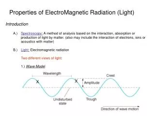
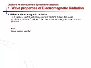
Chapter 6 An Introduction to Spectrometric Methods 1. Wave properties of Electromagnetic Radiation. 1.1 What ’ s electromagnetic radiation - a sinusoidal electric and magnetic wave traveling through the space

E N D
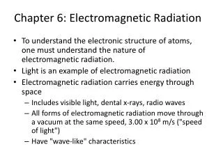
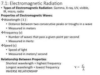
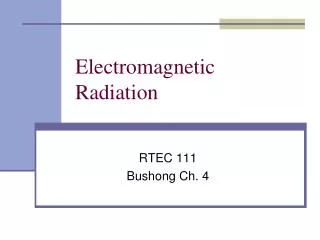
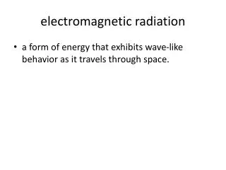
Chapter 6 An Introduction to Spectrometric Methods1. Wave properties of Electromagnetic Radiation 1.1 What’s electromagnetic radiation - a sinusoidal electric and magnetic wave traveling through the space - a discrete series of “particles” that have a specific energy but have no mass, photons Both. Wave-particle duality!
1.2 Wave properties of electromagnetic radiation (considering electric field only since it’s responsible for spectroscopy including transmission, reflection, refraction, and absorption) : wavelength, linear distance between two equivalent points on successive waves. A: amplitude, the length of electric vector at a maximum : frequency, the number of oscillations occurred per sec. T: period, time for 1 to pass a fixed point, =1/ y = A sin(t + ), with time as variable : angular velocity =2, : phase angle Coherent: a set of waves with identical and difference in phase angle remains constant y = A sin(t + ), y’ = A’sin(t + ’), - ’ = constant Fig. 6-1 (p.133)
1.2.1 Transmission velocity of wave propagation (m/s) = (m) x (s-1) - In a vacuum: electromagnetic wave travels at the speed of light, c = 3.00 x10⁸ m/s - In other media, remains constant, and thus v decreases v = c/n, n: the medium refractive index 1.00 1.2.2 Reflection and refraction The fraction of reflection: The extent of refraction:
1.2.3 Diffraction Parallel electromagnetic wave can be bend when passing through a narrow opening (width ). Fig. 6-7 (p.138)
Fig. 6-8 (p.139) Fig. 6-7 (p.138) Two diffracted rays from two slits will have interference. Constructive interference (intense band) can be observed when the difference in path length from two slits is equal to wavelength (first order interference), or 2, 3 … corresponding to difference between two phase angles = 2n, n is an integral 1,2,3…
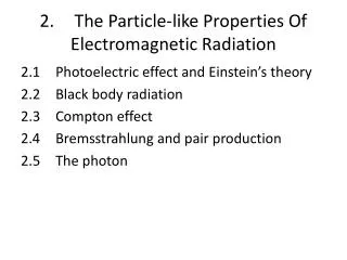
2. Particle Description of Radiation 2.1 Particle Properties According to Photoelectric Effect experiment (p144-146) energy of a photon can be related to its frequency E (J) = h h: Planck's constant, 6.6254 x10⁻³⁴ Js =c/ E = hc/ energy is inversely proportional to the wavelength
2.2 Some Commonly Used Units wavelength units vary with the spectral region X-ray and short UV: Å = 10-10 m UV/Visible range: nm = 10-9 m m = 10-6 m Infrared range: m wavenumber (cm-1): Photon energy X-ray region: eV 1J = 6.24 x10¹⁸ eV Visible region: kJ/mol kJ/mol = J/photon x6.02 x1023 photon/mol X10-3 kJ/J
2.2 Range of wavelength/frequencies Fig. 6-3 and Table 6-1 (p.135)
3 Interaction with Matter 3.1 Postulates of Quantum Mechanics • Atoms, ions and molecules exist in discrete energy states only -- quantized E0: ground E1, E2, E3 … : excited states Excitation can be electronic, vibrational or rotational Energy levels of atoms, ions or molecules are all different, Measuring energy levels gives means of identification of chemical species – spectroscopy • When an atom, ion or molecule changes energy state, it absorbs or emits radiation with energy equal to the energy difference E = E1 - E0 The wavelength or frequency of radiation absorbed or emitted during a transition
3.2 Emission Spectra from Excited States Fig. 6-15 (p.147) Sample is excited by the application of thermal, electrical or chemical energy Fig. 6-21 (p.151)
Fig. 6-23 (p.153) Measurement of the emitted radiation as a function of wavelength
3.3 Absorption Spectra Just as in emission spectra an atom, ion or molecule can only absorb radiation if energy matches separation between two energy states. Atoms No vibrational or rotation energy levels – sharp line spectra with few features Na 3s3p 589.0, 589.6 nm (yellow), For valence excitation, visible energy For core(inner) excitation, UV and X-ray energy
Fig. 6-16 (p.148) For absorption to occur, the energy of incident beam must be correspond to one of the energy difference 3s3p 589.0, 589.6 nm Fig. 6-23 (p.153) Measurement of the amount of light absorbed as a function of wavelength
Molecules Electronic, vibrational and rotational energy levels all involved – Each electronic state – many vibratioanl states Each vibrational states – many rotational states E = Eelec + Evib + Erot broad band spectra with many features. Fig. 6-23 (p.153)
3.4 Relaxation Processes Lifetime of excited state is short (fsms) – relaxation processes Nonradiative relaxation loss of energy by collisions, happens in a series of small steps. Tiny temperature rise of surrounding species Radiative relaxation (emission) Fluorescence (<10-5s) Stokes shift: emission has a lower frequency than the radiation (due to vibrational relaxation occurs before fluorescence).
Fast vibrational relaxation E2+e4”-E1 Stokes shift: emission has a lower frequency than the radiation due to vibrational relaxation occurs before fluorescence. E2-E1 Fig. 6-24 (p.154)
3.5 Quantitative aspects of spectrochemical measurements Assuming blank signal is already corrected for Emission Spectra S = kc Absorption Spectra Transmittance expressed as percent: T% = P/P0 x 100% Absorbance: A = -log10 T = log(P0/P) Beer’s Law A = bc : molar absorptivity (Lmol-1cm-1) b: path length of absorption (cm-1) C: molar concentration (mol L-1) Fig. 6-25 (p.158)