Fault Detection Tools and Techniques
Fault Detection Tools and Techniques. Fahmida N Chowdhury University of Louisiana at Lafayette. Jorge L Aravena Louisiana State University. White Box Approach. Black Box Approach . Gray Box Approach. FAULT DETECTION. Model/Residual Based. Model Free/DSP Based. Plant. Residual. Model.


Fault Detection Tools and Techniques
E N D
Presentation Transcript
Fault Detection Tools and Techniques Fahmida N Chowdhury University of Louisiana at Lafayette JorgeL Aravena Louisiana State University
White Box Approach Black Box Approach Gray Box Approach FAULT DETECTION Model/Residual Based Model Free/DSP Based
Plant Residual Model If a model is not available, must develop one using experimental data Modeling in Real Time
For TLRN, training issues are still open problems Input-output models (ARMA, ARMAX NARMA, NARMAX) State-space models [current work using time-lagged neural networks (TLRN)] • Backpropagation • through time (BPTT) • Kalman filter and • EKF-based training of • ANNs
Time-lagged neural network used for state space modeling W11 X1(k) a V1 W13 U(k-1) W21 Y(k) W12 W23 V2 Second-order example: can be generalized b X2(k)
y1(t) y2(t) y1(t) y2(t) t w11 w12 1 2 w22 w12 w11 … w22 1 2 w21 y2(t-1) y1(t-1) w21 t-1 1 2 w12 w11 w22 x1(t) x2(t) w21 y1(t-2) y2(t-2) t-2 1 2 x1(t-2) x2(t-2) The effect of Unfolding in BPTT
BPTT for RNN training Y0,Y1,Y2… Neural Net x0, x1, x2,... Neural Net DW average DW DW DW y0 y1 y2 x1 x2 x0 ... Back propagation
Extended Kalman Filter training • EKF is a state estimation technique for nonlinear systems derived by linearizing the well-known linear-systems Kalman filter around the current estimates. • In order to apply EKF to the task of estimating optimal weights of Recurrent Neural Networks(RNN), we interpret the weights of the network as the state of a dynamical system. x(n+1) = f(x(n), u(n)) + q(n) d(n) = hn(x(n)) w(n+1) = w(n) + q(n) d(n) = hn(w(n), u(n)) w : vector containing all the weights of the RNN. The output d(n) of the RNN is a function h of the weights and the input. The NN training task now takes the form of estimating the state from an initial guess w(0) and the sequence of outputs and inputs: d(0), …d(n), u(0), …, u(n).
EKF Algorithm for RNN training Predict Update
How good is the model that we just developed? Testing goodness of fit: Autocorrelation functions Chi-squared tests Kolmogoroff-Smirnov tests Under no-fault conditions, in the presence of only random disturbances, the residuals must be random
Kolmogoroff-Smirnov Test • H0: F(x) = F0(x) True, • H1: false Form the empirical estimate of F(x) and use as test statistic the maximum distancebetween F(x) and F0(x): q = max |F(x) – F0(x)| Find a constant c such that P{q>c|H0} = a Where a = 2exp(-2nc2) (Kolmogoroff approximation) Accept H0 iff q < sqrt[(-1/2n) ln(a/2)] = c a will be the probability of false alarm (type I error)
For uncertain systems, it cannot be guaranteed that residuals under no-fault conditions will be random! Many of our experimental models for arbitrary nonlinear plants showed non-perfect residuals: that is, the K-S test failed. Using these types of residuals would create many false alarms.
If there is a fault, then the residuals start to show systematic patterns These patterns may help us classify the various faults
Model/Residue Based Model Free/DSP Based White Box Approach Black Box Approach Gray Box Approach CWT & STFT Filter Banks FAULT DETECTION • You cannot correct what you cannot see • At the onset of a fault normal data is nuisance Model Free characterization in terms of changes in energy distribution • Signal Processing can eliminate nuisance data without requiring math models • “Enough” experimental data can replace a mathematical model • Unsupervised clustering does not require a model
Fault created here F14 SIMULINK MODEL
Input to DSP algorithms - filter bank in this case If residuals are not available??? By examining the sensor reading one cannot see the onset of the fault “Residuals”
(DASC2001) Onset is clear Some components show distinct pre - and post - fault behavior It may be possible to classify faults Faults cause changes in energy distribution
Pseudo Power Signature • Pseudo power signature Develop a signature that characterizes the energy distribution of a signal in a manner that is essentially independent of the duration of the signal.
Pseudo Power Signature • Time-frequency energy density function scalogram of a function with CWT (1) (2) The scalogram can be used as a time-frequency energy density function.
Signature subspace (DASC2002) Uses Singular Value Decomposition to approximate a function of two variables e.g. if two values are significant
Data generated with 1-axis model of F14 Things are beginning to get gray
If there is a fault, then the residuals start to show systematic patterns These patterns may help us classify the various faults
Things are getting whiter We can determine (unstable) poles of a system Required knowledge of input: it is bounded Strain sensor reading on airplane frame undergoing cycles of expansion (laboratory data) Second order model assumed and unstable pole used to characterize sensitivity of sensor
White sequence Uncorrelated! Decimated output has a pure AR model And Whiter • If the input is a stationary random process with a rational • spectrum we know we can ‘whiten’ input and have an • ARMAX model of the form Faster than Yule-Walker
How Useful Are Residuals? If there is no random noise in the system, residuals are very useful (FDI using parity check methods etc.) How to enhance the useful information hidden in the residuals If there is noise, residuals may be too fuzzy to use directly. AutoRegressive modeling of the residuals … AR parameters estimated by a Kalman filter in real time
Using the • IFAC Benchmark Problem for FDI • Ship Propulsion System • http://www.control.auc.dk/ftc/html/body_ship_propulsion_.html • Available Models- One Engine and one propeller • Two Engines and two propellers • Detailed Description of the Benchmark available in: • Izadi-Zamanabadi R. and M. Blanke (1999), A Ship Propulsion System Model for Fault-Tolerant Control, In Control Engineering Practice, 7(2), 227-239. • Izadi-Zamanabadi R. and M. Blanke (1998), A Ship Propulsion System as a Benchmark for Fault-tolerant Control, Technical report, Control Engineering Dept., Aalborg University
In the ship propulsion system, we introduced a slowly developing fault in the engine torque. The output is the ship speed, and the controller output is the fuel index. Residuals are collected at both the system output and controller output nodes. As expected, the controller output residuals are more sensitive (than the system output) to the fault.
The residuals are modeled with AR-Kalman-filter, and the AR-predicted residual signal shows drastically enhanced performance for early fault detection/warning. Issues in closed-loop FDI: in the presence of controllers, residuals at the system output becomes less sensitive to faults; the smarter the controller, the worse the output residuals!
Raw Residuals andAR-Predicted Values(controller output) Fault starts at time 12 sec.
Raw Residuals andAR-Predicted Values(system output) Fault starts at time 12 sec.
Using the AR-predicted residuals at the controller output appears to be the best option. If the residuals are purely random, then any attempt to fit AR or any other type of model must fail – essentially, the Kalman filter will then simply extract the zero signal from the noisy data. When a fault starts, the AR-parameters will shape up according to the type of the fault. All we need is an excellent real-time AR estimation tool.
Students: • Sundara Kumar (AR modeling, closed-loop FDI) • Venu Gopal Siddhanti (EKF for TLRN training) • Nageswara Rao (quality of residuals, hypothesis tests) • Dilip Vutukuru, Silpa Mutukuru, Karuna Pilla • (closed-loop FDI, smart controllers and FDI) Min Luo (FDI, Subspace signatures) Pallavi Chetan (STFT signatures, clustering) Santosh Desiraju (Detection of Change) James Henderson (Strain test data analysis)
for a switched system, the difference with respect to the ideal tracking performance corresponds to a combination of free responses from faulted and un-faulted systems and is essentially independent of the controller.