Transportation Problems
Transportation Problems. Joko Waluyo , Ir., MT., PhD Dept. of Mechanical and Industrial Engineering. Outline. Introduction. Solution Procedure for Transportation Problem. Finding an Initial Feasible Solution. Finding the Optimal Solution.

Transportation Problems
E N D
Presentation Transcript
Transportation Problems Joko Waluyo, Ir., MT., PhD Dept. of Mechanical and Industrial Engineering
Outline • Introduction • Solution Procedure for Transportation Problem • Finding an Initial Feasible Solution • Finding the Optimal Solution • Special Cases in Transportation Problems • Maximisation in Transportation Problems • Exercises
Operation Research • The main typical issues in OR : • Formulate the problem • Build a mathematical model • Decision Variable • Objective Function • Constraints • Optimize the model
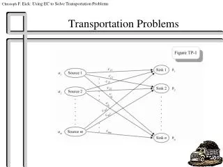
Introduction • Transportation models deal can be formulated as a standard LP problem. Typical situation shown in the manufacturer example • Manufacturer has three plants P1, P2, P3 producing same products. • From these plants, the product is transported to three warehouses • W1, W2 and W3. • Each plant has a limited capacity, and each warehouse has specific • demand. Each plant transport to each warehouse, but transportation • cost vary for different combinations. • The problem is to determine the quantity each warehouse in order to minimize total transportation costs.
Solution Procedure for Transportation Problem • Conceptually, the transportation is similar to simplex method. • Begin with an initial feasible solution. • This initial feasible solution may or may not be optimal. The only way you can find it out is to test it. • If the solution is not optimal, it is revised and the test is repeated. Each iteration should bring you closer to the optimal solution.
Solution Procedure for Transportation Problem • The format followed in the above table will be used throughout the unit. • Each row corresponds to a specific plant and each column corresponds to a specific warehouse. • Plant supplies are shown to the right of the table and warehouse requirements are shown below the table. • The larger box (also known as cells) at the intersection of a specific row and column will contain both quantity to be transported and per unit transportation cost. • The quantity to be transported will be shown in the centre of the box and will be encircled and the per unit transportation cost is shown in the smaller rectangular box at the left hand side corner.
Finding an Initial Feasible Solution There are a number of methods for generating an initial feasible solution for a transportation problem. Consider three of the following (i) North West Corner Method (ii) Least Cost Method (iii) Vogel’s Approximation Method
North West Corner Method (NWCM) The simplest of the procedures used to generate an initial feasible solution is NWCM. It is so called because we begin with the North West or upper left corner cell of our transportation table. Various steps of this method can be summarised as under. Step 1 Select the North West (upper left-hand) corner cell of the transportation table and allocate as many units as possible equal to the minimum between available supply and demand requirement i.e., min (S1, D1). Step 2 Adjust the supply and demand numbers in the respective rows And columns allocation.
Step 3 • If the supply for the first row is exhausted, then move down to the first cell in t he second row and first column and go to step 2. (b) If the demand for the first column is satisfied, then move horizontally to the next cell in the second column and first row and go to step 2. Step 4 If for any cell, supply equals demand, then the next allocation can be made in cell either in the next row or column. Step 5 Continue the procedure until the total available quantity id fully allocated to the cells as required.
Remark 1:The quantities so allocated are circled to indicated, the value of the corresponding variable. Remark 2:Empty cells indicate the value of the corresponding variable as zero, I.e., no unit is shipped to this cell. To illustrate the NWCM, As stated in this method, we start with the cell (P1 W1) and Allocate the min (S1, D1) = min (20,21)=20. Therefore we allocate 20 Units this cell which completely exhausts the supply of Plant P1 and leaves a balance of (21-20) =1 unit of demand at warehouse W1
Now, we move vertically downward to cell (P2 W1) At this stage the largest allocation possible is the (S2, D1 –20) =min (28, 1)= 1. This allocation of 1 unit to the cell (P1 W2). Since the demand of warehouse W2 is 25 units while supply available at plant P2 is 27 units, therefore, the min (27-5) = 25 units are located to the cell (P1 W2). The demand of warehouse W2 is now satisfied and a balance of (27-225) = 2 units of supply remain at plant P2. Moving again horizontally, we allocated two units to the cell (P2 W3) Which Completely exhaust the supply at plant P2 and leaves a balance of 17 units to this cell (P3, W3).. At this, 17 Units ae availbale at plant P3 and 17 units are required at warehouse W3. So we allocate 17 units to this cell (P3, W3). Hence we have made all the allocation. It may be noted here that there are 5 (+3+1) allocation which are necessary to proceed further. The initial feasible solution is shown below. The Total transportation cost for this initial solution is Total Cost = 20x7 +1 X 5 + 25 x 7 + 2 X 3 + 17 + 8 = Rs. 462
Least Cost Method • The allocation according to this method is very useful as it takes into consideration the lowest cost and therefore, reduce the computation as well as the amount of time necessary to arrive at the optimal solution. • Step 1 • Select the cell with the lowest transportation cost among all the rows or columns of the transportation table. • If the minimum cost is not unique, then select arbitrarily any cell with this minimum cost. • Step 2 • Allocate as many units as possible to the cell determined in Step 1 and eliminate that row (column) in which either supply is exhausted or demand is satisfied.
Repeat Steps 1 and 2 for the reduced table until the entire supply at different plants is exhausted to satisfied the demand at different warehouses.
Vogel’s Approximation Method (VAM) This method is preferred over the other two methods because the initial feasible solution obtained is either optimal or very close to the optimal solution. Step 1: Compute a penalty for each row and column in the transportation table. Step 2: Identify the row or column with the largest penalty. Step 3: Repeat steps 1 and 2 for the reduced table until entire supply at plants are exhausted to satisfy the demand as different warehouses.
Finding the Optimal Solution • Once an initial solution has been found, the next step is to test that solution for optimality. The following two methods are widely used for testing the solutions: • Stepping Stone Method • Modified Distribution Method • The two methods differ in their computational approach but give exactly the same results and use the same testing procedure.
Stepping-Stone Method • In this method we calculate the net cost change that can be obtained by introducing any of the unoccupied cells into the solution. • The Stepping Stone Method • Make sure that the number of occupied cells is exactly equal to m=n-1, where m=number of rows and n=number of columns. • Evaluate each unoccupied cells by following its closed path and determine its net cost change. • Determine the quality to be shipped to the selected unoccupied cell. Trace the closed path for the unoccupied cell and identify the minimum quality by considering the minus sign in the closed path.
Modified Distribution (MODI) Method The MODI method is a more efficient procedure of evaluating the unoccupied cells. The modified transportation table of the initial solution is shown below
Special Cases in Transportation Problem • Multiple Optimal Solutions • Unbalanced Transportation Problems • Degeneracy in Transportation Problem • Maximization In Transport Problems • Prohibited Routes
The initial feasible solution • North West Corner Rule • Least cost • Vogel’s Approach method • The Optimal solution • Stepping Stone Method • Modified Distribution Method
Example Problem
i = number of sources j = number of demands
Decision variable Number of millions energy (kWh) produced from sources and sent to demands x (i,j) = number of sources i = number of sources j = number of demands
Constraints • Constraints of number of Supply and demand x (i,j) > 0 (i = 1,2,3) and j=1,2,3,4) • Constraints of Supply • Constraints of Demands j = number of demands
Objective function • Minimize cost cost =
Model to be optimized cij = variable cost xij= number of unit transported from supply point i to demand j
Model to be optimized Objective function cij = variable cost xij= number of unit transported from supply point i to demand j
Review Questions and Exercises • What is unbalanced transport problem? • What is degeneracy? • Solve the following transportation problem.
Outlines • Introduction • Assignment Models. • Hungarian Method of Assignment Problems. • Special Cases in Assignment Problems. • Exercises
Introduction The Assignment problem deals in allocating the various items (resources) to various receivers (activities) on a one to one basis in such a way that the resultant effectiveness is optimised. Assignment Models This is a special case of transportation problem. In this problem, supply in each now represents the availability of a resource such as man, vehicle, produce, etc.
Hungarian Method of Assignment problem • An efficient method for solving an assignment problem, known as Hungarian method of assignment based on the following properties • In an assignment problem, if a constant quantity is added or subtracted from every element of any row or column in the given cost matrix, an assignment that minimizes the total cost in the matrix also minimize the total cost in the other. • In an assignment problem, a solution having zero total cost is an optimum solution. It can be summarized as follows. • Step 1:- In the given matrix, subtract the smallest element in each row from every element of the row. • Step 2:- Reduced matrix obtained from step1, subtract the smallest element in each column from every element of that column. • Step 3:- Make the assignment for the reduced matrix obtained from steps 1 and 2. • Continued ….
Step 4:-Draw the minimum number of horizontal and vertical lines to cover all zeros in the reduced matrix obtained from 3 in the following way. • Mark () all rows that do not have assignments. • Mark () all column that have zeros in marked rows (step 4 (a)). • Mark () all rows that have assignments in marked columns (step 4 (b)) • Repeat steps 4 (a) to 4 ( c ) until no more rows or columns can be marked. • Draw straight lines through all unmarked rows and marked columns. • Step 5:-If the number of lines drawn ( step 4 ( c ) are equal to the number of columns or rows, then it is an optimal solution, otherwise go to step 6. • Step 6:-Select the smallest elements among all the uncovered elements. • Step 7:-Go to step 3 and repeat the procedure until the number of assignments become equal to the number of rows or column.
Example A company faced with problem of assigning 5 jobs to 5 machines. Each job must be done on only machine. The cost of processing is as shown
Solution Now, select the minimum cost (element) in each row and subtract this element form each element of that row.
Special Cases in Assignment Problems • Maximization Cases. • Multiple Optimal Solution • 1. Maximization Cases :- • The Hungarian method explained earlier can be used for maximization case. The problem of maximization can be converted into a minimization case by selecting the largest element among all the element of the profit matrix and then subtracting it from all the elements of the matrix. We Can then proceed as usual and obtain the optimal solution by adding original values to the cells to which assignment have been made.
Multiple Optimal Solution: Sometimes, it is possible to have two or more ways to cross out all zero elements in the final reduced matrix for a given problem. This implies that there are more than required number of independent zero elements. In such cases, there will be multiple optimal solutions with the same total cost of assignment. In such type of situation, management may exercise their judgment or preference and select that set of optimal assignment which is more suited for their requirement. ….
Summary Assignment problem is a special case of transportation problem. It deals with allocating the various items to various activities on a one to one basis in such a way that the resultant effectiveness is optimised. In this unit, we have solved assignment problem using Hungarian Method. We have also disscussed the special cases in assignment problems.
Review Questions and Exercises. • What is an assignment problem? • Solve the assignment problem.