Confidence Intervals
Confidence Intervals. This chapter presents the beginning of inferential statistics. We introduce methods for estimating values of these important population parameters: proportions, means, and variances.

Confidence Intervals
E N D
Presentation Transcript
Confidence Intervals This chapter presents the beginning of inferential statistics. We introduce methods for estimating values of these important population parameters: proportions, means, and variances. We also present methods for determining sample sizes necessary to estimate those parameters.
Estimate a population Parameter • According to the U.S. Bureau of Labor Statistics, we earned average after-tax incomes of about $_________ per person in 2004 and spent about $________ per person. • Make an estimate of what the average after-tax income would be in 2004 • Now give your self a margin of error so you are 90% confident of your guess and give an interval that would capture the population. • Now give your self a margin of error so you are 70% confident of your guess. What is this interval? • Now give your self a margin of error so you are 50% confident of your guess. What is this interval? • What happened to the margin of error and the width of your intervals • http://www.time.com/time/nation/article/0,8599,1549403,00.html
According to the U.S. Bureau of Labor Statistics, we earned average after-tax incomes of about $22,000 per person in 2004 and spent about $17,000 per person.
DefinitionPoint Estimate • A point estimate is a single value (or point) used to approximate a population parameter. • The sample mean is the best point estimate of the population mean .
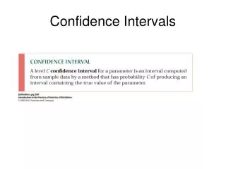
DefinitionConfidence Interval • A confidence interval (or interval estimate) is a range (or an interval) of values used to estimate the true value of a population parameter. A confidence interval is sometimes abbreviated as CI.
DefinitionConfidence Interval • A confidence level is the probability 1— (often expressed as the equivalent percentage value) that is the proportion of times that the confidence interval actually does contain the population parameter, assuming that the estimation process is repeated a large number of times. This is usually 90%, 95%, or 99%. ( = 10%), ( = 5%), ( = 1%)
DefinitionConfidence Interval • The confidence level is also called the degree ofconfidence, or the confidence coefficient. • Basically a 95% Confidence Interval means that if the survey was conducted many times that 95 % of the intervals would contain the actual population parameter.
DefinitionConfidence Interval • Or a 95% confidence interval implies that if 100 different samples were taken and the confidence intervals were constructed then we would expect 95% of them to include the parameter for the population. http://www.ruf.rice.edu/~lane/stat_sim/conf_interval/index.html
Assumptions • The sample is a simple random sample. All samples of the same size have an equal probability of being selected • The population is normally distributed or the sample size is n > 30 • The population standard deviation is known σ.
Critical Values • 1. We know from Chapter 8 that under certain conditions, the sampling distribution of sample means can be approximated by a normal distribution. • 2. Sample means have a relatively small chance (with probability denoted by ) of falling in one of the red tails of Figure 1 below • 3. Denoting the area of each shaded tail by /2, we see that there is a total probability of that a sample mean will fall in either of the two red tails. /2 /2
Critical Values • 4. By the rule of complements, there is a probability of 1— that a sample mean will fall within the inner region of Figure 1. • 5. The z score separating the right-tail iscommonlydenoted by z /2, and is referred to as a critical value because it is on the borderline separating sample means that are likely to occur from those that are unlikely to occur. See next slide.
= 5% 2 = 2.5% = .025 z2 -z2 Critical Values Finding z2for 95% Degree of Confidence 1- .95 =
z2 = 1.96 Finding z2for 95% Degree of Confidence = 0.05 Use Table A-4 to find a z score of 1.96
E = z/2 • n x - E Definition Margin of Error µ x + E also called the maximum error of the estimate
μ This confidence interval is not big enough to capture the population’s parameter μ
μ Depending on the size of the error E the confidence interval will contain the population parameter μ
x - E Definition Margin of Error is the maximum likely difference observed between sample mean x and true population mean µ. denoted by E µ x + E
x - E Definition Margin of Error is the maximum likely difference observed between sample mean x and true population mean µ. denoted by E µ x + E x -E < µ < x +E upper limit lower limit
E = z/2 • n x - E Definition Margin of Error µ x + E also called the maximum error of the estimate
Confidence Interval (or Interval Estimate) for Population Mean µ(Based on Large Samples: n >30) x - E < µ < x + E µ = x + E (x + E, x - E)
Lets return to the demonstration. http://www.ruf.rice.edu/~lane/stat_sim/conf_interval/index.html
x - E < µ < x + E Procedure for Constructing a Confidence Interval for µ( Based on a Large Sample: n > 30 ) 1. Find the critical value z2 that corresponds to the desired degree of confidence. 2. Evaluate the margin of error E = z2 • / n . If the population standard deviation is unknown, use the value of the sample standard deviation s provided that n > 30. (This method will be discussed later) 3. Find the values of x - E and x + E. Substitute those values in the general format of the confidence interval: 4. Round using the confidence intervals roundoff rules.
Round-Off Rule for Confidence Intervals Used to Estimate µ • When using the original set of data, round the confidence interval limits to one more decimal place than used in original set of data. 2. When the original set of data is unknown and only the summary statistics (n, x, s)are used, round the confidence interval limits to the same number of decimal places used for the sample mean.
Example: A study found the body temperatures of 106 healthy adults. The sample mean was 98.2 degrees and the sample standard deviation was 0.62 degrees. Find the margin of error E and the 95% confidence interval.
Example: A study found the body temperatures of 106 healthy adults. The sample mean was 98.2 degrees and the population standard deviation was 0.62 degrees. Find the margin of error E and the 95% confidence interval. n = 106 x = 98.20o σ = 0.62o = 0.05 /2 = 0.025 z/ 2= 1.96 E = z/ 2• = 1.96 • 0.62 = 0.12 n 106
Example: A study found the body temperatures of 106 healthy adults. The sample mean was 98.2 degrees and the sample standard deviation was 0.62 degrees. Find the margin of error E and the 95% confidence interval. n = 106 x = 98.20o s = 0.62o = 0.05 /2 = 0.025 z/ 2= 1.96 E = z/ 2• = 1.96 • 0.62 = 0.12 n 106 x - E < < x + E
Example: A study found the body temperatures of 106 healthy adults. The sample mean was 98.2 degrees and the sample standard deviation was 0.62 degrees. Find the margin of error E and the 95% confidence interval. n = 106 x = 98.20o s = 0.62o = 0.05 /2 = 0.025 z/ 2= 1.96 E = z/ 2• = 1.96 • 0.62 = 0.12 n 106 x - E < < x + E 98.20o - 0.12 <<98.20o + 0.12
E = z/ 2• = 1.96 • 0.62 = 0.12 n 106 x - E < < x + E Example: A study found the body temperatures of 106 healthy adults. The sample mean was 98.2 degrees and the sample standard deviation was 0.62 degrees. Find the margin of error E and the 95% confidence interval. n = 106 x = 98.20o s = 0.62o = 0.05 /2 = 0.025 z/ 2= 1.96 98.20o - 0.12 <<98.20o + 0.12 98.08o << 98.32o (98.08º ,98.32º )
E = z/ 2• = 1.96 • 0.62 = 0.12 n 106 x - E < < x + E Example: A study found the body temperatures of 106 healthy adults. The sample mean was 98.2 degrees and the sample standard deviation was 0.62 degrees. Find the margin of error E and the 95% confidence interval. n = 106 x = 98.20o s = 0.62o = 0.05 /2 = 0.025 z/ 2= 1.96 98.08o << 98.32o (98.08º ,98.32º ) Based on the sample provided, the confidence interval for the population mean is 98.08o<<98.32o. If we were to select many different samples of the same size, 95% of the confidence intervals would actually contain the population mean .
Finding the Point Estimate and E from a Confidence Interval Point estimate of µ: x =(upper confidence interval limit) + (lower confidence interval limit) 2
Finding the Point Estimate and E from a Confidence Interval Point estimate of µ: x =(upper confidence interval limit) + (lower confidence interval limit) 2 Margin of Error: E = (upper confidence interval limit) - (lower confidence interval limit) 2
x - E < < x + E Things to Remember • C.I. = Point Estimate ± margin of error • As the error gets bigger the C.I. increases • As n increases the error decreases • As σ increases the error increases

