Download
1 / 14
180 likes | 538 Vues
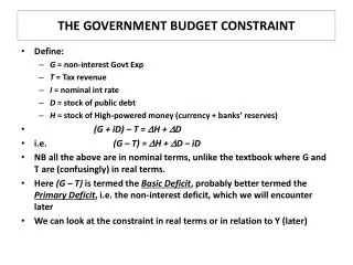
THE GOVERNMENT BUDGET CONSTRAINT. Define: G = non-interest Govt Exp T = Tax revenue I = nominal int rate D = stock of public debt H = stock of High-powered money (currency + banks’ reserves) (G + iD) – T = H + D i.e. (G – T) = H + D – iD

E N D
THE GOVERNMENT BUDGET CONSTRAINT • Define: • G = non-interest Govt Exp • T = Tax revenue • I = nominal int rate • D = stock of public debt • H = stock of High-powered money (currency + banks’ reserves) • (G + iD) – T = H + D • i.e. (G – T) = H + D – iD • NB all the above are in nominal terms, unlike the textbook where G and T are (confusingly) in real terms. • Here (G – T) is termed the Basic Deficit, probably better termed the Primary Deficit, i.e. the non-interest deficit, which we will encounter later • We can look at the constraint in real terms or in relation to Y (later)
CAUSES OF HYPERINFLATION • Sometimes a negative Supply Shock can start a process: normally real Y falls and P increases • If Wages are indexed to prices this can lead to further increases in P • A falling exchange rate can be a further channel for transmitting inflation • The same process can cause the Fiscal Deficit to increase: if this is financed by H, there is further impetus to inflation • Two key points: • the dependence on monetary financing requires a compliant Central Bank • lack of credibility on bond markets may increase recourse to monetary financing
EXTREME HYPERINFALTIONS • Country Peak Annual Rate Daily Rate Time to double • Hungary July 1946 1.30(1016) % 195 % 15.6 hours • Zimbabwe Nov 2008 7.96(1010) % 98 % 24.7 hours • Yugoslavia Jan 1994 3.13(108) % 64.6 % 1.4 days • Germany Nov 1923 29,500 % 20.9 % 3.7 days • Greece Nov 1944 11,300 % 17.1 % 4.5 days • China May 1949 4,210 % 13.4 % 5.6 days • Source: Prof. Steve H. Hanke, (Johns Hopkins University) • Note circumstances: wars, civil disruption.
STOPPING HYPERINFLATIONS • Reduce the (real) Budget deficit: • Expenditure • Tax revenues • Reduce/abandon indexation • Establish central bank independence • Link to external currency ($ ?): Currency board with 100 reserve backing • Establish credibility – a political issue • In some extreme cases a currency is abandoned de facto in response to hyperinflation (Zimbabwe?) • Many Latin American hyperinflations have been tamed only after several false starts: the effects may linger for a long time.
THE AFTER-EFFECTS OF HYPERINFLATIONS • Often we can assess credibility by looking at Government bond yields: compared with benchmark German Bunds and US Treasury bonds (approx 3.4% and 3.7% for 10-years as of July 2009) • Argentina: Stabilized in 92; Currency board 1Peso = 1$; breakdown indluding default in 2001 due to continuing fiscal deficits, inflation back up to 10-15%; 3-month int rate 14.63%; 25 year indexed Arg Peso bonds 16.7% • Brazil: stabilization in 94 (Real plan): in 2001 currency peg to $ abandoned, fiscal deficit controlled, inflation now 5.5%; 3-month int rate 9.16%; 1 year bond rate 8.97%; 10 yr $ bond yield 6.16% • Chile: Inflation of 1,300% by 1973; stabilization under military rule in late ’70s; subsequent banking crisis; inflation now 4%; 3-month int rate 1.32%; 10-year indexed Cl.Peso bond yield 2.83%; 10 yr $ bond yield 3.07%
FISCAL DEFICITS AND DEBIT IN THE LONG-RUN • Governments often run budget deficits • Persistent deficits imply a build-up of debts • How sustainable is any fiscal policy in the long-run? • Presumably what really matters - just as for any individual borrower - is the ratio of Debt to Income (or GDP) • This in turn is related to: • (i) the size of the fiscal deficit in relation to GDP • (ii) the rate of growth of GDP • (iii) the interest rate at which the Government can borrow • (iv) the rate of return on investments financed by government borrowing – which of course may affect (ii)
A SIMPLE MODEL OF DEFICITS AND DEBT (1) • Let: B = conventional (fiscal) deficit (Gen Govt Deficit) P = Primary Deficit (i.e. non-Interest Deficit) G = Govt. non-interest Expenditure D = Stock of Govt. Debt i = Interest rate (Nominal): r = real int rate T = Govt (Tax) Revenue gn, g = nominal and real growth rates of GDP The subscript t refers to time • Bt Dt D t-1 or Dt • Also Bt (i Dt-1 + Gt ) –Tt • Initially assume Y is constant • Stabilising D Y in this case holding D constant
A SIMPLE MODEL OF DEFICITS AND DEBT (2) • i.e. Bt = Dt = 0 • or, (i Dt-1 + Gt ) – Tt = 0 • and, i Dt-1 = (Tt – Gt ) = (–)Pt • One must have a Primary Surplus equal to the Debt Interest costs. If not, one has to borrow to cover (part of) the interest..... • The Primary (or non-interest) Surplus is (T - G), which is the negative of the Primary Deficit, (G - T) • Taking i Dt-1 = (Tt Gt ) = – Pt as a ratio of Y: • i (D/Y) = (T G)/Y = – P/Y • The required Primary Surplus depends on the initial D Y and on the interest rate, i • When Y is growing (at a rate of gn%), this will be amended. By itself, a growing Y will lower (D Y) and make stabilization easier • The initial term is then (i - gn)(D Y) • The static example is just a special case where gn = 0 • Clearly in real terms we have (r – g)(D/Y)
A SIMPLE MODEL OF DEFICITS AND DEBT (3) • i (D/Y) = (T G) • For an economy where the nominal growth rate is gn, the stabilizing D/Y requires that D/D < or = Y/Y • i.e B = D = (Y/Y)D = gnD • Basically: (D/Y) = D/Y (D/Y)gn (1) • and D = G + iD – T • D/Y = G/Y + i(D/Y) – T/Y (2) • Sub (2) into (1): (D/Y) = G/Y + i(D/Y) – T/Y (D/Y)gn (3) • i.e. (D/Y) = (G – T)/Y + (i – gn)(D/Y) • For stable (D/Y) i.e. (D/Y) = 0 this implies: • (T – G)/Y = (i – gn)(D/Y) • Or in real terms: (T – G)/Y = (r – g)(D/Y)
DEFICITS, DEBT: POLICY (1) • Case A: IRL now, Italy (90s) ? • Case B: Italy post EMU ? • Case C: Ireland 2006 07 ? • Case D: US 2014 ?
DEFICITS, DEBT: POLICY (2) • Post 2014: assume real growth 3%, inflation 2%, interest rate 5%, initial D/Y = 1.3 • This implies (gn – i) = 0 and therefore P/Y should be = 0 to maintain D/Y constant • As Debt interest i(D/Y) = 0.05(0.8) = 0.04, there will have to be a Fiscal Deficit of no more than 4% of GDP • The EU Stability and Growth pact originally had a 3% fiscal deficit ceiling. Also a D/Y ceiling of 60% • Cyclical v structural deficits
THE GOVERNMENT BUDGET CONSTRAINT • Government expenditure is financed either by taxation or by borrowing, but borrowing implies future taxes • Formally: PV(G) = PV(T) • In a 2-period model: • G1 + G2(1+r) = T1 + T2 (1+r) • i.e. G1T1 = (T2 G2 )(1+r) • or T2 = (G1 T1 )(1+r) + G2 • Expected future taxes increase with present deficits (G1T1)or expected future Govt expenditures (G2) • Implication: suppose the Government implements a tax cut financed by an increase in borrowing • Households are better off now, but is they foresee future taxes increasing, this will offset the tax cut • Result: Increase in Sp offsets reduction in Sg
RICARDIAN EQUIVALENCE (1) • More realistically (2010), suppose a very large increase in the Government deficit is expected in the next 4 years • Rationally, households expect large tax increases and reductions in future disposable income. • Result: possible large increases in Sp, which of course will reduce government revenue from expenditure taxes, etc…. • Recent developments: USA; Ireland where Sg has turned strongly negative, but Current a/c deficit of BOP has reduced significantly: implication Sp must have increased (Sp + Sg = BOP) • The Barro-Ricardo equivalence theorem throws doubt on the efficacy of discretionary fiscal policy. • While there are some historical episodes which might support it there are also severe doubts:
RICARDIAN EQUIVALENCE (2) • Are government bonds net wealth? No, if Barro is right. • But do people discount the future at a higher rate than the long-term bond rate? If so, then the theorem falls • Empirically there are doubts: e.g. US tax cuts in the 80s and 2000s have been associated with reduced personal savings, contrary to the theorem (assuming unchanged government expenditures and hence larger deficits, people should have expected future tax increases and saved more in the present…) • However the Irish fiscal correction of the late 80s was not accompanied by the deflation feared by some: did private consumption and investment expand in response to lower expected taxes and higher expected disposable incomes?