Chapter 10: Aggregate Demand I
Chapter 10: Aggregate Demand I. The IS-LM Model. A short-run macroeconomic model which takes the price level constant and shows how changes in the level of Aggregate Demand cause changes in income. The IS curve: The Keynesian Cross Theory


Chapter 10: Aggregate Demand I
E N D
Presentation Transcript
The IS-LM Model • A short-run macroeconomic model which takes the price level constant and shows how changes in the level of Aggregate Demand cause changes in income. • The IS curve: The Keynesian Cross Theory • The LM curve: The Liquidity Preference Theory
Shift in Aggregate Demand An increase in the level AD increases the level of income, given the price level. Price level P SRAS AD3 AD2 AD1 Y1 Y2 Y3 Output, Income
The Keynesian Cross Equilibrium in the product market: • Planned Expenditures: E = C(Y-T) + I + G • Actual Expenditures: Y • Aggregate Equilibrium: Y = C(Y-T) + I + G Total income = Total planned expenditures
Aggregate Equilibrium Actual Expenditure: Y = E E Planned Expenditure: E = C + I + G Keynesian Cross Increase inventories Reduce inventories Y2 Y Y1 Y
Adjustment to Equilibrium • Y1> Y indicates an excess supply of goods in the market. So, businesses accumulate inventories to reduce Y1 to Y • Y2<Y indicates an excess demand for goods in the market. So, businesses reduce inventories to increase Y2 to Y
Effect of Stabilization Policy • A government policy of changing planned expenditure, C, I, or G, would shift the Planned Expenditure line to increase the level of income. • The increase in income is subject to a multiplier effect as spending by consumers receiving the new income, creates income for other consumers
Effect of Government Spending Policy Y = E E = C + I + G2 E E = C + I + G1 ΔG B A ΔY Y1 Y2 Y
Government Spending Multiplier • ΔG = Increase in government purchases • ΔY = Increase in income • Multiplier effect: ΔY / ΔG = 1 / (1 – MPC) • Example, MPC = 0.6, Spending Multiplier = 2.50; Any $1 increase in G creates an additional $2.50 of income
Effect of Government Tax Policy Y = E E = C2 + I + G E E = C 1+ I + G ΔC B A ΔY Y1 Y2 Y
Government Tax Multiplier • ΔT = Decrease in income taxes • ΔC = Increase in consumption = -MPC * ΔT • ΔY = Increase in income • Multiplier effect: ΔY / ΔT = -MPC / (1 – MPC) • Example, MPC = 0.6, Tax Multiplier = -1.50; Any $1 decrease in T creates an additional $1.50 of income
Derivation of IS Curve • IS shows level of income and interest rate that bring about equilibrium to the product market • Assume an initial income level and interest rate. An increases in interest rate reduces planned investment. Then, the Planned Expenditure line shifts down, causing income to decline.
IS Curve Interest rate IS shows pairs of income and interest rate such as (Y1, r1) and (Y2, r2) that bring about equilibrium in the product market. The higher the interest rate, the lower the level of income. r2 B A r1 Y2 Y1 Income
Shift of IS Curve Interest rate An increase in planned expenditure (C, I, or G) causes the IS to increase, hence increasing the level of income through the multiplier effect. IS2 IS1 Income Y2 Y1
Theory of Liquidity Preference • Equilibrium in the money market • Demand for money: (M/P)d = L(r,Y) • Money supply: (M/P)s = M/P • Equilibrium: M/P = L(r, Y)
Money Market Equilibrium _ M/P r r1 L(r, Y) M/P
Derivation of LM Curve • An increase in the level of income causes the demand for money to increase. As a result of a higher demand for money, the interest rate goes up • The higher the level of income, the higher is the rate of interest
Derivation of LM Curve LM shows pairs of income and interest rate such as (Y1, r1) and (Y2, r2) that bring bout equilibrium in the money market. _ M/P r LM r2 r2 r1 r1 L(r, Y2) L(r, Y1) Y1 Y2 M/P
Shift in LM Curve LM1 M1/P M2/P r LM2 r1 r1 r2 r2 L(r, Y) Y M/P An increase in the money supply, lowers the interest rate, making the LM curve to increase.
Aggregate Equilibrium • Aggregate equilibrium is achieved when IS = LM • IS: Y = C(Y - T) + I(r) + G • LM: M/P = L(r, Y)
Aggregate Equilibrium Interest rate LM r IS Y Income
Theory of Short-Run Fluctuations AD Curve Keynesian Cross IS Curve Short-run Fluctuations: Income Interest Rate AD-AS Model IS-LM Model Theory of Liquidity Preference LM Curve AS Curve