Seismic Observations of Mantle Interfaces: Insights from Global Studies
This study by Peter Shearer explores the seismic observations of different mantle interfaces, focusing on their origins and properties. It distinguishes between consistently observed interfaces (e.g., 410 km, 520 km, and 660 km) and those that are intermittently observed or hypothesized. The research utilizes data from various sources to analyze interface depths, seismic reflections, and precursor studies, shedding light on the complex geology of the Earth's mantle. The findings suggest potential undiscovered regional reflectors and emphasize the linked roles of mineral physics and geodynamics in understanding mantle structure.

Seismic Observations of Mantle Interfaces: Insights from Global Studies
E N D
Presentation Transcript
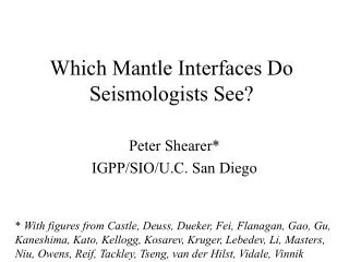
Which Mantle Interfaces Do Seismologists See? Peter Shearer* IGPP/SIO/U.C. San Diego * With figures from Castle, Deuss, Dueker, Fei, Flanagan, Gao, Gu, Kaneshima, Kato, Kellogg, Kosarev, Kruger, Lebedev, Li, Masters, Niu, Owens, Reif, Tackley, Tseng, van der Hilst, Vidale, Vinnik
Interface Depth vs. Publication Date Most depths are sampled at least once Consistency in depths greatest for 220, 410, 520, 660 Note: plot is not complete, especially in last 15 years
Three Types of Mantle Interfaces Routinely observed seismically, known mineral physics origin (410, 520, 660) Intermittently observed seismically, undetermined origin (220, 900, 1200, D”) Unobserved seismically, hypothesized by geochemists or geodynamicists (e.g., Kellogg et al. lower mantle boundary)
SS precursors probe layering near the SS bounce point Nice for global studies since SS bounce points are widely distributed
410 and 660 observations are consistent with mineral physics predictions for olivine phase changes • Absolute depths agree with expected pressures • Topography consistent with Clapeyron slopes • Size of velocity and density jumps are about right figure from Lebedev et al. (2002)
• Correlation between TZ thickness and velocity anomalies • Agrees with mineral physics data for olivine phase changes • Permits calibration of dT/dv and Clapeyron slopes Australia region, Receiver functions Global, SS precursors Flanagan& Shearer (1998) Lebedev et al. (2002)
Analysis of different discontinuity phases can resolve density, P & S velocity jumps across discontinuities A puzzle: Where is the 660 reflector?
Estimated S velocity and density jumps across 660 km Global Study Northwest Pacific Philippine Sea Shearer & Flanagan (1999) SS & PP precursors Kato & Kawakatsu (2001) ScS reverberations Tseng & Chen (2004) Triplicated waveforms
Eastern US, MOMA Array Snake River Plane Dueker & Sheehan (1997) Li et al. (1998)
Tibet Tanzania Owens et al. (2000) Kosarev et al. (1999)
Southern Africa Gao et al. (2002)
P’P’ phase: seen at short periods, good for sharpness constraints
Comparison to long-period reflections Corrected for attenuation
No visible 410 in P’P’ at higher frequencies from Fei, Vidale & Earle
Conclusions from Fei, Vidale & EarleP’P’ study 410 is not so sharp — results suggest half is sharp jump, half is spread over 7 km 520 is not seen in short-period reflections — jump must occur over 20 km or more 660 is sharp enough to efficiently reflect 1 Hz P-waves — less than 2-km thick transition
S520S Seen in global stacks but weaker than 410 and 660 reflectors
SS precursors stacked in bounce point caps 520-km discontinuity may be intermittent and/or split into two interfaces Deuss & Woodhouse propose this may be phase changes in two components, olivine and garnet, whose depths don’t always coincide. Deuss & Woodhouse (2001)
Transects of the 520 Lateral continuity of structure
A global map, where there is coverage John Woodhouse
Three Types of Mantle Interfaces Intermittently observed seismically, undetermined origin (220, 900, 1200, D”)
Are there regional reflectors hidden in here, such as the 220?
SS Precursor Stacks in Different Regions figure from Deuss & Woodhouse (2002)
Discontinuity depths in SS precursor bounce point caps figure from Deuss & Woodhouse (2002)
But another SS precursor study does not find N. American 220 figures from Gu, Dziewonski & Ekstrom (2001)
Are there regional reflectors hidden down here, such as at 900 km or 1200 km?
Strongest evidence for mid-mantle discontinuities is from S-to-P conversions from deep earthquakes to receiver
• Interface near 1000 km below Indonesia • Seen in S-to-P conversions Slide 44 figures from Niu & Kawakatsu (1997)
• Interface near 1500 km below Marianas • Seen in S-to-P conversions below deep earthquakes figure from Kaneshima & Helffrich (1999)
Three Types of Mantle Interfaces Unobserved seismically, hypothesized by geochemists or geodynamicists (e.g., Kellogg et al. lower mantle boundary)
Hypothesized Undulating Mid-Mantle Discontinuity Low density contrast (chemical+thermal) implies large dynamic topography figures from Kellogg, Hager, van der Hilst (1999)
Some tomography models may have change in character near 1700 km depth But this is not direct evidence for an interface, and models have limited resolution and uniqueness…. figure from van der Hilst & Karason (1999)
Tackley (2002) test of Kellogg et al. hypothesized layer • 3-D numerical simulation of mantle convection • Filtered to match seismic modeling • Simulations predict peak in heterogeneity near interface depth • Not seen in real tomography models – argues against hypothesis Interface position Temperature perturbation
Radial correlation function is measure of vertical continuity of model Convection simulations with dense lower layer predict significant de-correlation (narrowing) near interface, which is not observed in Masters or Grand tomography models Seismic Inversion Convection Simulations Masters et al. model 10% in dense layer 30% in dense layer figures from Tackley (2002)
Thermal boundary layer at interface will cause sharp velocity change, which should cause observable triplication in seismic travel time curve* * Provided source/receiver geometry is just right figure from Vidale, Schubert & Earle (2001)
• California network data, 10 earthquakes • No triplications or complicated waveforms • But approach could miss: - interface not at 1770 km, or - dipping interface figures from Vidale, Schubert & Earle (2001)
S-to-P conversions can detect discontinuities below earthquake source regions S1700P phase arrives between P and pP Useful for finding interfaces below subduction zones from ~800 to ~2000 km depth figure from Castle & van der Hilst (2003)
Systematic search for interfaces below Pacific subduction zones Nothing 1500 - 1800 km (see also Wicks & Weber, 1996; Kaneshima & Helffrich, 1999) Nothing Nothing figure from Castle & van der Hilst (2003)
Yet Vinnik et al. study finds interfaces in some of same places 1200 km 900 km 1850 km 950 & 1050 km 1200 km figure adapted from Vinnik, Kato & Kawakatsu (2001)
S1200P S1700P s410P Quake in Fiji-Tonga, recorded in Japan Quake in Marianas, recorded in western US figure from Vinnik, Kato & Kawakatsu (2001)
What about the lowermost mantle? figure from Castle & van der Hilst (2003)
• Mid-mantle reflectors seen below many subduction zones • Related to ancient slabs? • Discontinuity observations lacking in other areas • Not present? or Not easy to observe? • Conclusion: Seismic evidence argues against continuous mid-mantle boundary