Download
1 / 30
300 likes | 410 Vues
Learn about decomposing directed acyclic graphs into minimum node-disjoint chains, essential in compressing partial orders and solving transitive closures. This paper presents the algorithm and applications of graph decomposition.

E N D
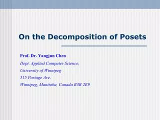
On the Graph Decomposition Yangjun Chen and Yibin Chen Dept. Applied Computer Science, University of Winnipeg 515 Portage Ave. Winnipeg, Manitoba, Canada R3B 2E9
Outline • Motivation • Graph stratification • Main algorithm - Bipartite graphs and virtual nodes - Chain generation - Resolving virtual nodes • Summary
Motivation • Graph decomposition into node-disjoint chains Given a directed acyclic graphG, decompose it into a minimum set of node-disjoint chains, which cover all the nodes of G. For any two nodes u and v on a chain, if u is above v then there is a path from u to v in G. • Application - Decomposition of a partially ordered sets (posets) into a minimum set of chains - Compress transitive closures of graphs
Motivation a2 a1 a2 a1 a1 a2 a3 a3 a4 a3 a4 a4 a6 a5 a6 a5 a5 a6
Motivation Compression of transitive closures a1 a2 index Index sequence 1 2 a1 a3 a2 (1, 1) (2, 1) (1, 1)(2, 2) (1, 2)(2, 1) a4 (1, 1) a3 a4 (2, 2) (1, 2)(2, 2) (1, 3)(2, 2) a5 a6 a5 a6 (1, 3) (2, 3) (1, 3) (2, 3) O(n2) O(n) - number of chains
Main idea of graph decomposition • Stratifying a graph into a series of bipartite graphs: G1, …, Gh. • Finding a maximum matching Mi for each Gi. (In this process, virtual nodes may be introduced.) • Combining all Mi’s to get a set of chains, denoted as M1 … Gh, which may contain virtual nodes. • Removing the virtual nodes to get the final result.
Graph stratification Definition 1 Let G(V, E) be a DAG. We decompose V into subsets V0, V1, ..., Vh such that V = V0 V1 ... Vh and each node in Vi has its children appearing only in Vi-1, ..., V0 (i = 1, ..., h), where h is the height of G, i.e., the length of the longest path in G. q r s q r s V4: p n o m V3: n o p m j k l t i j k l t i V2: f g h x h V1: x f g b y c d e z a z a b y d e c V0:
Graph stratification Dividing a graph into a series of bipartite graphs: q r s V4: q r s V3: n o p m V3: n o p m n o p m j k l t i V2: j k l t i j k l t i V2: f g h x V1: f g h x a z b y d e c f g h V1: x V0: a z b y d e c
Virtual nodes Find a maximum matching for each bipartite graph and then combine them together, by which ‘virtual node’ may be introduced. Definition 2 (virtual nodes) Let G(V, E) be a DAG, divided into V0, ..., Vh (i.e., V = V0 ... Vh). Let Mi be a maximal matching of B(Vi, Vi-1′; Ci) for i = 1, …, h. For each free node v in Vi-1′ with respect to Mi, a virtual node v′ created for v is a new node added to Vi (1 i h - 1), denoted as v = s(v′).
Virtual Nodes Definition 2 (virtual nodes) Let G(V, E) be a DAG, divided into V0, ..., Vh (i.e., V = V0 ... Vh). Let Mi be a maximal matching of B(Vi, Vi-1′; Ci) for i = 1, …, h. For each free node v in Vi-1′ with respect to Mi, a virtual node v′ created for v is a new node added to Vi (1 i h - 1), denoted as v = s(v′). q r s V4: g h V1: x V3: n o p m V0: a z b y d e c j k l t i V2: g h M1: x V1’: g x c’ h e’ z’ f a z b y d e c label(t e’) = 0 label(j e’) = 1 label(t z’) = 0 label(k c’) = 1 label(i e’) = 0 label(k e’) = 1 label(i z’) = 0 label(l c’) = 1 label(j c’) = 1 label(l e’) = 1
Virtual Arcs inherited arcs- If there is u Vj (j > i) such that u v E, add uv′, referred to as an inherited arc. transitivearcs- If there exist u Vj (j > i) and w Vi such that uw E and wvCi, add uv′ if it has not been created as an inherited arc, referred to as a transitive arc. alternating arcsof the first kind - If there exists a covered node wVi-1′ (relative to Mi) such that one of v’s parents is connected to w through an -segment in B(Vi, Vi-1′; Ci), and u Vj (j > i) such that one of the two conditions holds: • uwE, or • there is a node w′ Visuch that uw′ E and w′wCi, add uv′ if it has not been created as an inherited or a transitive arc.
Chain Generation g h M1: x j k l t i M2: g h V1: x a z b y d e c g x c’ h e’ z’ f V0: a z b y d e c q r s M3: n o p m V4: V2: j k l t i q r s M4: j k l t i V3: n o p m V1’: o p e’ g x c’ h z’ f j k l t i V2: V1’: g x c’ h e’ z’ f
e Chain Generation q r s M4: o p q r s g h M1: x n o p m a z b y d e c j k l t i j k l t i M2: M3: n o p m g x c’ h e’ z’ f g x c’ h e’ z’ f j k l t i a z b y c d
e Chain Generation q r s q r s n o p m n o p m j k l t i j k l t i g x h f g x c’ h e’ z’ f a z b y c d e a z b y c d
Chain Generation q r s q r s n o p m n o p m j k l t i j k l t i g x h f g x h f a z a z b y c d e b y c d e
Chain Generation Definition 3 (alternating graph) Let B(T, S; E) be a bipartite graph. Let M be a matching of B(T, S; E). The alternating graph with respect to M is a directed graph with the following sets of nodes and arcs: = V( ) = TS, and = E( ) = {u v | uS, vT, and (u, v) M} {v u | uS, vT, and (u, v) E\M}. g h g h V1: V1: x x V0: V0: a a z z b y d e b y d e c c g h M1: x a z b y d e c
Chain Generation Next, we will combine two consecutive alternating graphs = (Vi′, Vi-1′; Ci) and = (Vi+1, Vi′; Ci+1), denoted as , by connecting each node in Vi+1 to all its reachable nodes in Vi-1′. j k l t i V2: V1: g x h f g x h f V1: V0: a z y c d e b
Chain Generation j k l t i V2: j k l t i V1: g x h f g x h f V1: g x h f g x h f V0: a z y c d e b a z y c d e b A maximum set of node disjoint paths with each starting from a free node u relative to Mi+1 in Vi+1, and ending at a free node v relative to Miin Vi-1′,
Chain Generation What we want is to find a maximum set S of node-disjoint paths in , each starting from a free node u relative to Mi+1 in Vi+1, and ending at a free node v relative to Miin Vi-1′. Let P be such a path with u and v being the starting and ending nodes. We will create a virtual node v´ for v, connect it u. However, for each free node (in Vi-1′) not appearing on such a path, its virtual node will be added to Vi+1, for which only inherited and transitive arcs, as well as a new kind of virtual arcs, called alternating arcs of the second kind will be created.
Chain Generation • Alternating arc of the second kind – Let v´ be a virtual node • Created for v in Vi-1′ and added to Vi+1. If there exist a free • node wVi-1′ (relative to Mi) and a node u Vj (j > i) such that • one of v’s parents is connected to w through a -segment in • B(Vi′, Vi-1′; Ci), satisfying one of the following two conditions: • - uwE, or • there is an alternating path in (Vi′, Vi-1′; Ci), which does not • go through any node in S, but connects w to a node x Vi-1′ • such that x is reachable from u, • add uv′ if it has not been created as an inherited or a • transitive arc. label(uv′)is set to be i, same as an • alternating arc incident to a virtual node added to Vi′.
V4: V3: V2: V1: V0: Chain Generation M2: j k l t i c′ q r s q r s x h g e′ z′ f n o p m n o c′′ p m M3: j k l t i c′ j k l t i c′ n o p m g h x e′ z′ f j k l t i c′ g h z′ x e′ f a z b y d e c M4: a z b y d e c q r s label(l e’) = 1 label(m c’) = 1 label(t z) = 0 label(q c’) = 1 label(q c) = 1 n o p m
Chain Generation q r s q r s V4: q r s n o c′′ p m c′′ n o p m n o c′′ p m V3: j k l t i c′ j k l t i c′ g h q r s x z′ e′ f M4: g h z′ x e′ f c′′ a z n o p m b y d e c a z b y d e c
Virtual Node Resolution • After the chain generation, the next step is to resolve • (or say, to remove) virtual nodes from chains. For this purpose, • we will work top-down along the chains. Two steps will be • carried out: • Remove virtual nodes, and at the same time connect some • nodes according to the connectivity represented by them, and • Establish new connections between free nodes by transferring • edges along alternating paths within a bipartite graph or cross • more than one bipartite graph.
Virtual Node Resolution When we try to remove virtual nodes v with label(u v) = i, all the virtual nodes with higher labels must have been eliminated. In this step, the following operations will be conducted. • Let v be a virtual node in Vi′. If v does not have a parent along • the corresponding chain, it will be simply removed. • If v has a parent u along a chain with label(uv) = 0, • remove v and connect u to s(v). label(us(v)) is set to 0. • Let level(s(v)) = i. Connect u to each reachable node in Vi.
Virtual Node Resolution • If v has a parent u along a chain with label(uv) = i, • remove v and connect u to each reachable node in Vi-1. • Construct a combined graph in a way similar to the chain • generation, involving the corresponding bipartite graphs, • where the direction of each arc corresponding to an edge • belonging to a maximum matching is reversed.
Virtual Node Resolution q r s q r s n o p m n o p m j k l t i j k l t i g h x f g h z′ x e′ f a z b y d e c a z b y d e c
Virtual Node Resolution q r s q r s n o p m n o p m j k l t i j k l t i j k l t i g h x f g f x h g a z b y d e f x h c a z b y d e c
Virtual Node Resolution q r s q r s n o c′′ p m n o p m j k l t i j k l t i c′ g h g h z′ x x e′ f f a a z z b y d e b y d e c c
Summary A efficient algorithm for graph decomposition - Graph stratification - Algorithm for finding maximum matching for bipartite graphs - Virtual nodes Computational complexities time: O(max{ n, m}) space overhead: O(n)