Download
1 / 58
580 likes | 619 Vues
Explore data simulation and analysis methods for understanding photospheric flows in solar physics research, addressing key questions and conclusions from Doppler velocity studies.

E N D
Characterizing Photospheric Flows David Hathaway (NASA/MSFC) with John Beck & Rick Bogart (Stanford/CSSA) Kurt Bachmann, Gaurav Khatri, & Joshua Petitto (Birmingham Southern College) Sam Han & Joseph Raymond (Tennessee Technological University) Åke Nordlund (Astronomical Observatory, Denmark) and of course Phil Scherrer and the MDI Team
OUTLINE • Why bother? • Simulating Photospheric Flow Data • MDI Data • Data Preparation: p-mode filtering • Axisymmetric Flow Analysis • The Convection Spectrum (Poloidal Component) • Radial Flow Component • Toroidal Flow Component • Angular Momentum Flux by Cellular Flows • Rotation Rates • Lifetimes • Conclusion
THREE BIG QUESTIONS IN SOLAR PHYSICS 1) What causes solar flares, prominence eruptions, and CMEs? 2) What causes the 11-year cycle of Sunspots and solar activity? 3) How is the corona heated and the solar wind accelerated?
Data Simulation • Calculate vector velocities using input spectrum of complex spectral coefficients, R, S, and T (Chandrasekhar, 1961). • Project vector velocities into the line-of-sight and integrate over pixels to get Doppler velocity signal
Data Simulation - Continued The resulting Doppler velocity signal is convolved with a point-spread-function representing the MDI optical system in Full Disk mode to simulate MDI Doppler velocity data. The final Doppler image is analyzed using the same processes used on the MDI data and results are compared to determine the complex spectral coefficients and their dependence upon ℓ and time.
This gets mapped onto heliographic coordinates and projected onto spherical harmonics to give spherical harmonic spectral coefficients.
Power Spectrum from the 61-day Sequence The peak at ℓ~120 represents supergranules with typical size λ ~ 2πR/ℓ ~ 36 Mm
Velocity Spectrum from the 61-day Sequence The peak at ℓ~140 represents supergranules with typical size λ ~ 2πR/ℓ ~ 31 Mm and typical Doppler velocity ~ 100 m/s
Data Simulation #1 This simulation only includes horizontal, poloidal flows with: and random phases, m.
Low Resolution High Resolution
Photospheric Convection Spectrum Conclusions • There is a continuous spectrum of convective flows from giant cells to granules • There are only two distinct modes of convection in the photosphere – granulation and supergranulation
Radial Flow Component Study The line-of-sight velocity at a point, (x,y), on the disk is given by: where ρ is the heliocentric angle from disk center with: and a second horizontal component, Vh2, is transverse to the line-of-sight.
Radial Flow Component Study If we consider the average mean-squared velocity at an angle ρ from disk center we find:
Exclude Magnetic Elements (|B| > 25 G)
Radial Flow Component Study Results We must include a radial component to the spectrum of the cellular flows with Rℓ=(0.05 + 0.07 ℓ/1000)Sℓ.
Radial Flow Study Conclusions • Radial flow is ~10% of the horizontal flow for supergranules (increases to ~15% for cells 4000 km across) • Doppler velocities under-estimate the horizontal flow speed by ~1.4
Toroidal Flow Study Solenoidal flows have strong radial gradients and weak tangential gradients. Toroidal flows have weak radial gradients and strong tangential gradients. Foreshortening near the limb weakens the radial gradients more than the tangential gradients. Solenoidal and toroidal flows will have different center-to-limb behavior. Radial Tangential
Toroidal Flow Study (Data Simulation w/o MTF) Solenoidal only – solid line, Toroidal only – dashed line
Toroidal Flow Study Comparison with MDI Data MDI – solid line, Data Simulation (30% Toroidal) – dashed line
Toroidal Flow Study Conclusions • Toroidal flow ~30% of the horizontal flow is consistent with data (but effects of MTF must be determined) • Phase relationship between Solenoidal and Toroidal components needs to be determined
Angular Momentum Transport • Axisymmetric flow (the meridional circulation) transports angular momentum toward the poles • Non-axisymmetric flows (cellular flows) can transport angular momentum toward the equator if prograde velocities (u') are correlated with equatorward velocities (v')
A Doppler Velocity Indicator ofAngular Momentum Transport Gilman (A&A 1977) showed that the mean squared Doppler velocity signal should be stronger east of the central meridian for an equatorward transport of angular momentum. Coriolis force on flows in east-west cells gives poleward transport and stronger Doppler signal west of the CM.. Coriolis force on flows in north-south cells gives equatorward transport and stronger Doppler signal east of the CM.
Cell Shape Analysis Compare observed spectral amplitudes as a function of m/ℓ for MDI data and simulated data. Simulated data has no preferred cell shape.
Angular Momentum Study Conclusions • Angular momentum is transported toward the poles in supergranules (instrumental problems – focus variations across disk and astigmatism – may severely impact this result)
Cross-Correlation Technique Cross-correlating strips at the same latitude gives the shift (rotation rate) required to give maximum correlation (lifetime).
Rotation Rate vs. Feature Size As the size of the features increases the rotation rate increases.
Data Simulation Rotation Rate vs. Feature Size As the size of the features increases the rotation rate increases.