4. Actuator and payload
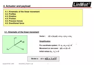
z. r (t). y. x. 4. Actuator and payload. 4.1. Kinematic of the linear movement 4.2. Profiles 4.3. Kinetics 4.4. Friction 4.5. Process forces 4.5. Gravitional force. 4.1. Kinematic of the linear movement. Vector : r (t) := [x,y,z] = x e x + y e y + z e z Simplification

4. Actuator and payload
E N D
Presentation Transcript
z r(t) y x 4. Actuator and payload 4.1. Kinematic of the linear movement 4.2. Profiles 4.3. Kinetics 4.4. Friction 4.5. Process forces 4.5. Gravitional force 4.1. Kinematic of the linear movement Vector : r(t) := [x,y,z] = x ex + y ey + z ez Simplification . . . Fix coordinate system: ex = ey = ez = 0 Movement on one axes: y(t) = z (t) = 0 Initial values (x0 , vo ) = 0 Stroke s: r(t) := x(t) = ½ a*t2
x(t) x(t) t t v(t) v(t) t t a(t) a(t) t t 4.1. Kinematic of the linear movement „short stroke movement‘ ‚long stroke movement‘ x(t) = ½ a*t2 x(t) = ½ a*t2 with v(t) < vmax with v(t) limited to vmax vmax • Estimation through x(t) = ½ a*t2 or Moving time t:= sqr(2x/ a) is only accurate if the motor is running beneath its velocity maximum • Be careful: vmax is load dependant • Estimats using x(t):= vmax * t or Moving time t:= x/ vmax do not take into account the acceleration phase of the movement • Be careful: vmax is load dependant State of the art sizing programs calculate the motion under the consideration within limitations of maximum velocities at load.
x(t) t v(t) t x a(t) t 4.2. Profile (1) Example of a simple pick and place two axes situation vmax ? stroke
4.2. Profile (2) • Case a: • Goal: moving time := 0 s • Infinite high a and v values • No real situation („Starship Enterprise‘ • Case b: • Goal: constant moving velocity • Infinite high acceleration values • Note: linear motors often can not implement their max acceleration due to system mechanics. In real world application most often the acceleration of linear motors have to be limited because of the shock and the stress produced on the mechanics.
4.2. Profile (3) • Case c: • Goal: constant acceleration with limitation to vmax • ‚Trapezoidal profile‘ • ‚ramp ‘ function of the velocity • Jerk because of step chance in acceleration mechanical stress . a • Case d: • Goal: ‚minimal jerk‘ profile • Linear increase of the acceleration • Derivation of the acceleraion is limited minimal stress to the mechanics • ‚extremely smooth movement‘ • Disadvantage: the movement needs a high acceleration at high velocity. Linear motor prefer to produce the highest acceleration during the time of low velocity (force/velocity diagram). Minimizing power required.
4.2. Profile (4) • Case e: • Goal: „Profile for general purpose“: Sine-profile • The highest acceleration is needed at velocity 0 m/s which is perfect for the behavior of linear motors.
x 4.2. Profile (5) Depending on the application it makes sense to use different profiles for different situations. State of the art linear motor systems offer such possibilities. E.g.: - sine-profile, if no product is gripped - minimal jerk profile, if a product is gripped and should be moved gently -.... Return movement with product ‚minimal jerk‘ movement without product ‚sine-profile‘
4.3. Kinetics: movement and force Newton‘s second law F:= Mass * acceleration = m * a [N] The inertial force is the most important force in dynamic (horizontal) applications. A higher machine trouh requires higher acceleration rates! Help: a) reduce mass of the construction ( Fe = 7,9 kg/dm3, Al = 2.7 kg/dm3, POM =1,4 kg/dm3 ) b) Optimize the profiles ( reduce max accelerations required) Note: F ~ m a reduction of the mass will reduce the needed motor force proportionally. F ~ a ~ 1/t2 A reduction of the moving time (Formula: x(t) = ½ a*t2 ) will increase the needed force by square! ( „double as fast 4 time higher accelerations are needed. if a machine is required to become faster it is critically important to optimize the mechanical construction)
Stiction /Break away friction Stiction leads to jerk movements of open loop systesm (e.g. Pneumatic cylinder).Closed-loop systems like linear motor will compensate the stiction effects! Dry friction Friction between two solid materials (caloric friction). FRt := * Fn = * m *g cos Viscous friction proportional to v (stirring a soup faster requires more force) F m Stiction FRt Fn Dry friction t a t 4.4. Friction Friction increases the force requirement during the phases of movement. Friction will lead to higher continuous force requirements.
4.5. Process forces Process forces appear most often during a certain time and/or location of the movement cycle.The most often seen examples are: F s s Springs ( testing of switches) Assembling forces ( assembling of parts) Pressing forces- labeling- stamping- painting Using state of the art sizing programs it is possible to simulate any process force during the single phases of the movement cycle.
1 kg Fg = 9.8 N 4.6. Gravitational forces (1) In vertical application (z-axes) this leads to a constant force in direction of the earth: Fg:= m * a = m * g with g = 9,81 m/s2. Drives with high stiction (ball screws with high pitch low velocity) this effect is not as important as with direct drives. Direct drives (rotating and linear) must produce a continuous force equal and opposite of thegravitanional force to produce zero accelerations (maintaining the position). There exists different options to compensate for Gravitational forces in vertical applications.
m mg m m m 4.6. Gravitational forces / Compensation (2) Pneumatic cylinder Constant pressure on the pneumatic cylinder will producea constant (stroke independant) force to compensate the weight. Counterbalance spring In real world applicationslimited to short strokes • Counterbalance mass (elevator) • if /a/> g dual connected cables • Will double the moved mass !
F s 4.6. Gravitational forces / MagSpring (3) • MagSpring™ (magnetic spring) • MagSprings, unlike mechanical springs, deliver a constant force over their entire wide working range. • MagSpring consists of only two rugged components: a stator and a slider. • MagSprings are totally electrically passive. Their operation is based entirely on a unique (patent pending) application of permanent magnets - no electricity at all. • Adventages • constant force over long stroke, force is not stroke depandant as a spring • High force in relation to the size (E.g..: 20 mm cylinder F= 20 N compensate 2 kg payload)small additional mass ( usable for high dynamic movements) • only two parts simplistic construction • passive element ! www.MagSpring.com m
4.6. Gravitational forces / Brake (4) Mechanical brakes for linear movements Mechanical brakes can be used as a mechanical stop in case of power loss. Mechanical brake for standard linear guide/rail. (Picture: Kendrion/Binder Magnettechnik)