Climate data

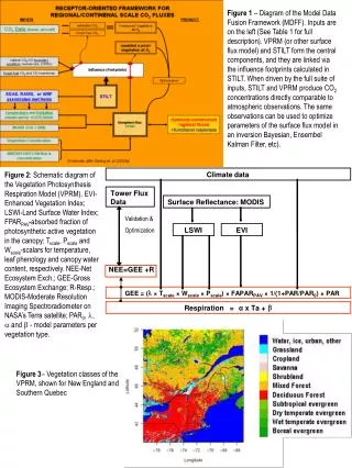
1. Figure 1 – Diagram of the Model Data Fusion Framework (MDFF). Inputs are on the left (See Table 1 for full description). VPRM (or other surface flux model) and STILT form the central components, and they are linked via the influence footprints calculated in STILT. When driven by the full suite of inputs, STILT and VPRM produce CO2 concentrations directly comparable to atmospheric observations. The same observations can be used to optimize parameters of the surface flux model in an inversion Bayesian, Ensembel Kalman Filter, etc). Figure 2: Schematic diagram of the Vegetation Photosynthesis Respiration Model (VPRM). EVI-Enhanced Vegetation Index; LSWI-Land Surface Water Index; FPARPAV-absorbed fraction of photosynthetic active vegetation in the canopy; Tscale, Pscale and Wscale-scalars for temperature, leaf phenology and canopy water content, respectively. NEE-Net Ecosystem Exch.; GEE-Gross Ecosystem Exchange; R-Resp.; MODIS-Moderate Resolution Imaging Spectroradiometer on NASA’s Terra satellite; PAR0,,  and  - model parameters per vegetation type. Climate data Tower Flux Data Surface Reflectance: MODIS Validation & LSWI EVI Optimization NEE=GEE +R  l GEE = ( × T × W × P ) × FAPAR × 1/(1+PAR/PAR ) × PAR scale scale scale PAV 0  b Respiration = α x Ta + Figure 3– Vegetation classes of the VPRM, shown for New England and Southern Quebec

2. a. b. c. e. d. Fig. 4(a,b) Comparison of observed (solid-square) and predicted (open-circle) hourly mean NEE (micromole/sqr.m/s) over the peak photosynthetically active period at calibration (a) and cross validation (b) sites (Parameters from NOBS, HARVARD, and HOWLAND were used to SOBS, INDIANA and LCREEK, respectively). (c,d) Same as (a,b), but for monthly mean NEE. (e) Linear regression analysis between observed and predicted monthly mean NEE (micromole/sqr.m/s) for all 12 cross validations sites (no optimization of parameters).

3. Figure 5 -- Series of monthly mean a priori flux estimates as calculated by the VPRM for New England and Southern Quebec. Figure 6 – Examples of how aircraft data helps evaluate and constrain modeling and synthesis activities (a) Comparison of PBL height calculated by RAMS with aircraft data, demonstrating RAMS generally capturing PBL height adequately. (b) Comparison of airborne free tropospheric CO2 concentrations and the advected boundary condition used in the MDFF (see Gerbig et. al. 2003b)). If the background condition were perfect, all points would fall on the 1:1 line.

4. Figure 7 (a) Average footprint <<f>> for the GMD Argyle Tall Tower in central Maine for the month of August 2004. Based on this footprint, Argyle measurements contain aggregated information about fluxes in Maine and Southern Quebec (b) Composite footprint for COBRA-2003 airborne campaign, demonstrating continental scale coverage Figure 8 a–(a) Hourly timeseries of the Argyle tall tower CO2 concentration as observed (black line) and calculated by the MDFF (red line).We stress that these use VPRM parameters are not optimized with atmospheric information, and rely only on the initial calibration with Ameriflux eddy covariance data. The a priori MDFF capture the day-to-day variations well. (b) Seasonal timeseries of the Argyle tall tower CO2 concentration as observed (black line) and calculated by the MDFF (red line) for May 15-September 15, 2004. Each point represents an afternoon average, with one point per day.The model background is shown in light grey for both plots Figure 8b--Direct comparison of model calculated values and observations. Both observations and model output were averaged over (a) morning (0800 to 1230 local time) and (b) afternoon (1230 to 1630 local time). The MDFF captures the observed variation in CO2 concentrations significantly better in the afternoon, likely a result of more reliable transport parameterizations in the meteorological products used as input (in this case EDAS-40).

5. Figure 9-West-to-east flight transect from the afternoon of 11-June-2004 showing (a) airborne in-situ CO2 concentrations (b) MDFF output along the flight path (c) the difference between the a and b. The difference between model and observation is in general smaller than the gradient observed in the atmosphere. Aircraft in-situ a priori STILT+VPRM Difference (obs – model) ppm CO2 a b c August NEE f d e e Figure 10-Preliminary regional budgets for New England and Quebec for 2004 (COBRA-Maine). (a-d) Monthly mean carbon flux (mmole m-2s-1) from the VPRM a priori surface flux model, driven by EDAS winds and solar radiation. (e, f)Change in AGB from forest inventories, with harvest added back in, for 1985-1995, and annual NEP (positive=uptake) from the ED-2 model driven by ECMWF meteorology [D. Medvigy and P. Moorcroft, private communication]. Spruce budworm damage is evident in N. Maine and Quebec(g) Net annual balance over the region in 2004 from the VPRM a priori.(note opposite sign convention: uptake=negative). Sunshine has a strong positive bias in the EDAS driver, compared to Harvard and Howland AmeriFlux data, leading to excessive uptake. A better sunshine product, from GOES or NLDAS, will be incorporated before optimizing a priori parameters vs constraints from Argyle tower data (Fig.8), inventories, and ED-2. g