Download
1 / 44
440 likes | 546 Vues
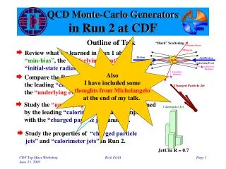
This talk reviews findings from CDF Run 1 regarding "minimum bias", the "underlying event", and initial-state radiation, while contrasting them with new data from Run 2. It explores variations in the underlying event definition using leading charged particle jets and calorimeter jets, studying multiple parton interactions. By comparing new insights with PYTHIA Tune A, the analysis aims to clarify the distinctions between hard and soft scattering processes and their correlations with charged particle density.

E N D
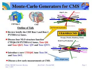
QCD Monte-Carlo Generatorsin Run 2 at CDF Also I have included some thoughts from Michelangelo at the end of my talk. Outline of Talk • Review what we learned in Run 1 about “min-bias”, the “underlying event”, and “initial-state radiation”. • Compare the Run 1 analysis which used the leading “charged particle jet” to define the “underlying event” with Run 2 data. Compare with PYTHIA Tune A • Study the “underlying event” in Run 2 as defined by the leading “calorimeter jet” and compare with the “charged particle jet” analysis. • Study the properties of “charged particle jets” and “calorimeter jets” in Run 2. JetClu R = 0.7 Rick Field
The “Underlying Event”in Hard Scattering Processes “Min-Bias” • What happens when a high energy proton and an antiproton collide? • Most of the time the proton and antiproton ooze through each other and fall apart (i.e.no hard scattering). The outgoing particles continue in roughly the same direction as initial proton and antiproton. A “Min-Bias” collision. Are these the same? • Occasionally there will be a “hard”parton-parton collision resulting in large transverse momentum outgoing partons. Also a “Min-Bias” collision. No! • The “underlying event” is everything except the two outgoing hard scattered “jets”. It is an unavoidable background to many collider observables. “underlying event” has initial-state radiation! Rick Field
Beam-Beam Remnants Maybe not all “soft”! • The underlying event in a hard scattering process has a “hard” component (particles that arise from initial & final-state radiation and from the outgoing hard scattered partons) and a “soft?” component (“beam-beam remnants”). • Clearly? the “underlying event” in a hard scattering process should not look like a “Min-Bias” event because of the “hard” component (i.e.initial & final-state radiation). • However, perhaps “Min-Bias” collisions are a good model for the “beam-beam remnant” component of the “underlying event”. Are these the same? • The “beam-beam remnant” component is, however, color connected to the “hard” component so this comparison is (at best) an approximation. Rick Field
MPI: Multiple PartonInteractions • PYTHIA models the “soft” component of the underlying event with color string fragmentation, but in addition includes a contribution arising from multiple parton interactions (MPI) in which one interaction is hard and the other is “semi-hard”. • The probability that a hard scattering events also contains a semi-hard multiple parton interaction can be varied but adjusting the cut-off for the MPI. • One can also adjust whether the probability of a MPI depends on the PT of the hard scattering, PT(hard) (constant cross section or varying with impact parameter). • One can adjust the color connections and flavor of the MPI (singlet or nearest neighbor, q-qbar or glue-glue). • Also, one can adjust how the probability of a MPI depends on PT(hard) (single or double Gaussian matter distribution). Rick Field
CDF Run 1 “Min-Bias” DataCharged Particle Density • Shows CDF “Min-Bias” data on the number of charged particles per unit pseudo-rapidity at 630 and 1,800 GeV. There are about 4.2 charged particles per unit h in “Min-Bias” collisions at 1.8 TeV (|h| < 1, all PT). <dNchg/dh> = 4.2 <dNchg/dhdf> = 0.67 • Convert to charged particle density, dNchg/dhdf, by dividing by 2p. There are about 0.67 charged particles per unit h-f in “Min-Bias” collisions at 1.8 TeV (|h| < 1, all PT). 0.67 0.25 • There are about 0.25 charged particles per unit h-f in “Min-Bias” collisions at 1.8 TeV(|h| < 1, PT > 0.5 GeV/c). Rick Field
CDF Run 1 “Min-Bias” DataPT Dependence Lots of “hard” scattering in “Min-Bias”! • Shows the energy dependence of the charged particle density, dNchg/dhdf, for “Min-Bias” collisions compared with HERWIG “Soft” Min-Bias. • Shows the PT dependence of the charged particle density, dNchg/dhdfdPT, for “Min-Bias” collisions at 1.8 TeV collisions compared with HERWIG “Soft” Min-Bias. • HERWIG “Soft” Min-Bias does not describe the “Min-Bias” data! The “Min-Bias” data contains a lot of “hard” parton-parton collisions which results in many more particles at large PT than are produces by any “soft” model. Rick Field
No easy way to “mix” HERWIG “hard” with HERWIG “soft”. Min-Bias: Combining“Hard” and “Soft” Collisions HERWIG diverges! sHC PYTHIA cuts off the divergence. Can run PT(hard)>0! • HERWIG “hard” QCD with PT(hard) > 3 GeV/c describes well the high PT tail but produces too many charged particles overall. Not all of the “Min-Bias” collisions have a hard scattering with PT(hard) > 3 GeV/c! HERWIG “soft” Min-Bias does not fit the “Min-Bias” data! • One cannot run the HERWIG “hard” QCD Monte-Carlo with PT(hard) < 3 GeV/c because the perturbative 2-to-2 cross-sections diverge like 1/PT(hard)4? Rick Field
PYTHIA Min-Bias“Soft” + ”Hard” Tuned to fit the “underlying event”! PYTHIA Tune A CDF Run 2 Default 12% of “Min-Bias” events have PT(hard) > 5 GeV/c! 1% of “Min-Bias” events have PT(hard) > 10 GeV/c! • PYTHIA regulates the perturbative 2-to-2 parton-parton cross sections with cut-off parameters which allows one to run with PT(hard) > 0. One can simulate both “hard” and “soft” collisions in one program. Lots of “hard” scattering in “Min-Bias”! • The relative amount of “hard” versus “soft” depends on the cut-off and can be tuned. • This PYTHIA fit predicts that 12% of all “Min-Bias” events are a result of a hard 2-to-2 parton-parton scattering with PT(hard) > 5 GeV/c (1% with PT(hard) > 10 GeV/c)! Rick Field
“Underlying Event”as defined by “Charged particle Jets” Look at the charged particle density in the “transverse” region! Charged Particle Df Correlations PT > 0.5 GeV/c |h| < 1 • Look at charged particle correlations in the azimuthal angle Df relative to the leading charged particle jet. • Define |Df| < 60o as “Toward”, 60o < |Df| < 120o as “Transverse”, and |Df| > 120o as “Away”. • All three regions have the same size in h-f space, DhxDf = 2x120o = 4p/3. “Transverse” region is very sensitive to the “underlying event”! Toward-side “jet” (always) Perpendicular to the plane of the 2-to-2 hard scattering Away-side “jet” (sometimes) Rick Field
Factor of 2! Run 1 Charged Particle Density“Transverse” PT Distribution • Compares the average “transverse” charge particle density with the average “Min-Bias” charge particle density (|h|<1, PT>0.5 GeV). Shows how the “transverse” charge particle density and the Min-Bias charge particle density is distributed in PT. PT(charged jet#1) > 30 GeV/c “Transverse” <dNchg/dhdf> = 0.56 “Min-Bias” CDF Run 1 Min-Bias data <dNchg/dhdf> = 0.25 Rick Field
ISAJET 7.32“Transverse” Density ISAJET uses a naïve leading-log parton shower-model which does not agree with the data! • Compares the average “transverse” charge particle density (|h|<1, PT>0.5 GeV) versus PT(charged jet#1) and the PT distribution of the “transverse” density, dNchg/dhdfdPT with the QCD hard scattering predictions of ISAJET 7.32 (default parameters with PT(hard)>3 GeV/c) . • The predictions of ISAJET are divided into three categories: charged particles that arise from the break-up of the beam and target (beam-beam remnants), charged particles that arise initial-state radiation, and charged particles that arise from the outgoing jets plus final-state radiation.. ISAJET Beam-Beam Remnants Initial-State Radiation Rick Field
ISAJET 7.32“Transverse” Density ISAJET uses a naïve leading-log parton shower-model which does not agree with the data! • Plot shows average “transverse” charge particle density (|h|<1, PT>0.5 GeV) versus PT(charged jet#1) compared to the QCD hard scattering predictions of ISAJET 7.32 (default parameters with PT(hard)>3 GeV/c) . • The predictions of ISAJET are divided into two categories: charged particles that arise from the break-up of the beam and target (beam-beam remnants); and charged particles that arise from the outgoing jet plus initial and final-state radiation(hard scattering component). ISAJET “Hard” Component Beam-Beam Remnants Rick Field
HERWIG 6.4“Transverse” Density HERWIG uses a modified leading-log parton shower-model which does agrees better with the data! • Plot shows average “transverse” charge particle density (|h|<1, PT>0.5 GeV) versus PT(charged jet#1) compared to the QCD hard scattering predictions of HERWIG 5.9(default parameters with PT(hard)>3 GeV/c). • The predictions of HERWIG are divided into two categories: charged particles that arise from the break-up of the beam and target (beam-beam remnants); and charged particles that arise from the outgoing jet plus initial and final-state radiation(hard scattering component). HERWIG “Hard” Component Beam-Beam Remnants Rick Field
HERWIG 6.4“Transverse” PT Distribution HERWIG has the too steep of a PT dependence of the “beam-beam remnant” component of the “underlying event”! • Compares the average “transverse” charge particle density (|h|<1, PT>0.5 GeV) versus PT(charged jet#1) and the PT distribution of the “transverse” density, dNchg/dhdfdPT with the QCD hard scattering predictions of HERWIG 6.4(default parameters with PT(hard)>3 GeV/c. Shows how the “transverse” charge particle density is distributed in PT. Herwig PT(chgjet#1) > 30 GeV/c “Transverse” <dNchg/dhdf> = 0.51 Herwig PT(chgjet#1) > 5 GeV/c <dNchg/dhdf> = 0.40 Rick Field
PYTHIA: Multiple PartonInteraction Parameters and now HERWIG! Pythia uses multiple parton interactions to enhance the underlying event. Jimmy: MPI J. M. Butterworth J. R. Forshaw M. H. Seymour Multiple parton interaction more likely in a hard (central) collision! Same parameter that cuts-off the hard 2-to-2 parton cross sections! Hard Core Rick Field
Tuning PYTHIA:Multiple Parton Interaction Parameters Hard Core Determine by comparing with 630 GeV data! Affects the amount of initial-state radiation! Take E0 = 1.8 TeV Reference point at 1.8 TeV Rick Field
PYTHIA 6.206 Defaults MPI constant probability scattering PYTHIA default parameters • Plot shows the “Transverse” charged particle density versus PT(chgjet#1) compared to the QCD hard scattering predictions of PYTHIA 6.206 (PT(hard) > 0) using the default parameters for multiple parton interactions and CTEQ3L, CTEQ4L, and CTEQ5L. Default parameters give very poor description of the “underlying event”! Note Change PARP(67) = 4.0 (< 6.138) PARP(67) = 1.0 (> 6.138) Rick Field
Tuned PYTHIA 6.206 Tune A CDF Run 2 Default! Double Gaussian PYTHIA 6.206 CTEQ5L • Plot shows the “Transverse” charged particle density versus PT(chgjet#1) compared to the QCD hard scattering predictions of two tuned versions of PYTHIA 6.206 (CTEQ5L, Set B (PARP(67)=1)and Set A (PARP(67)=4)). Old PYTHIA default (more initial-state radiation) Old PYTHIA default (more initial-state radiation) New PYTHIA default (less initial-state radiation) New PYTHIA default (less initial-state radiation) Rick Field
Azimuthal Correlations PYTHIA Tune A (more initial-state radiation) PYTHIA Tune B (less initial-state radiation) • Predictions of PYTHIA 6.206 (CTEQ5L) with PARP(67)=1 (new default) and PARP(67)=4 (old default) for the azimuthal angle, Df, between a b-quark with PT1 > 15 GeV/c, |y1| < 1 and bbar-quark with PT2 > 10 GeV/c, |y2|<1 in proton-antiproton collisions at 1.8 TeV. The curves correspond to ds/dDf (mb/o) for flavor creation, flavor excitation, shower/fragmentation, and the resulting total. Rick Field
Azimuthal Correlations PYTHIA Tune A (more initial-state radiation) • Predictions of HERWIG 6.4 (CTEQ5L) for the azimuthal angle, Df, between a b-quark with PT1 > 15 GeV/c, |y1| < 1 and bbar-quark with PT2 > 10 GeV/c, |y2|<1 in proton-antiproton collisions at 1.8 TeV. The curves correspond to ds/dDf (mb/o) for flavor creation, flavor excitation, shower/fragmentation, and the resulting total. PYTHIA Tune B (less initial-state radiation) “Flavor Creation” Rick Field
Tuned PYTHIA 6.206“Transverse” PT Distribution PT(charged jet#1) > 30 GeV/c Can we distinguish between PARP(67)=1 and PARP(67)=4? No way! Right! PARP(67)=4.0 (old default) is favored over PARP(67)=1.0 (new default)! • Compares the average “transverse” charge particle density (|h|<1, PT>0.5 GeV) versus PT(charged jet#1) and the PT distribution of the “transverse” density, dNchg/dhdfdPT with the QCD Monte-Carlo predictions of two tuned versions of PYTHIA 6.206 (PT(hard) > 0, CTEQ5L, Set B (PARP(67)=1)and Set A (PARP(67)=4)). Rick Field
Tuned PYTHIA 6.206Run 1 Tune A Describes the rise from “Min-Bias” to “underlying event”! Set A PT(charged jet#1) > 30 GeV/c “Transverse” <dNchg/dhdf> = 0.60 “Min-Bias” Set A Min-Bias <dNchg/dhdf> = 0.24 • Compares the average “transverse” charge particle density (|h|<1, PT>0.5 GeV) versus PT(charged jet#1) and the PT distribution of the “transverse” and “Min-Bias” densities with the QCD Monte-Carlo predictions of a tuned version of PYTHIA 6.206 (PT(hard) > 0, CTEQ5L, Set A). Describes “Min-Bias” collisions! Describes the “underlying event”! Rick Field
“Transverse” Charged Particle Density “Transverse” region as defined by the leading “charged particle jet” • Shows the data on the average “transverse” charge particle density (|h|<1, PT>0.5 GeV) as a function of the transverse momentum of the leading charged particle jet from Run 1. Excellent agreement between Run 1 and 2! • Compares the Run 2 data (Min-Bias, JET20, JET50, JET70, JET100) with Run 1. The errors on the (uncorrected) Run 2 data include both statistical and correlated systematic uncertainties. PYTHIA Tune A was tuned to fit the “underlying event” in Run I! • Shows the prediction of PYTHIA Tune A at 1.96 TeV after detector simulation (i.e. after CDFSIM). Rick Field
“Transverse” Charged PTsum Density “Transverse” region as defined by the leading “charged particle jet” • Shows the data on the average “transverse” charged PTsum density (|h|<1, PT>0.5 GeV) as a function of the transverse momentum of the leading charged particle jet from Run 1. Excellent agreement between Run 1 and 2! • Compares the Run 2 data (Min-Bias, JET20, JET50, JET70, JET100) with Run 1. The errors on the (uncorrected) Run 2 data include both statistical and correlated systematic uncertainties. PYTHIA Tune A was tuned to fit the “underlying event” in Run I! • Shows the prediction of PYTHIA Tune A at 1.96 TeV after detector simulation (i.e. after CDFSIM). Rick Field
“Underlying Event”as defined by “Calorimeter Jets” Charged Particle Df Correlations PT > 0.5 GeV/c |h| < 1 Look at the charged particle density in the “transverse” region! • Look at charged particle correlations in the azimuthal angle Df relative to the leading JetClu jet. • Define |Df| < 60o as “Toward”, 60o < |Df| < 120o as “Transverse”, and |Df| > 120o as “Away”. • All three regions have the same size in h-f space, DhxDf = 2x120o = 4p/3. “Transverse” region is very sensitive to the “underlying event”! Perpendicular to the plane of the 2-to-2 hard scattering Away-side “jet” (sometimes) Rick Field
“Transverse” Charged Particle Density “Transverse” region as defined by the leading “calorimeter jet” • Shows the data on the average “transverse” charge particle density (|h|<1, PT>0.5 GeV) as a function of the transverse energy of the leading JetClu jet (R = 0.7, |h(jet)| < 2) from Run 2. , compared with PYTHIA Tune A after CDFSIM. • Compares the “transverse” region of the leading “charged particle jet”, chgjet#1, with the “transverse” region of the leading “calorimeter jet” (JetClu R = 0.7), jet#1. Rick Field
“Transverse” Charged PTsum Density “Transverse” region as defined by the leading “calorimeter jet” • Shows the data on the average “transverse” charged PTsum density (|h|<1, PT>0.5 GeV) as a function of the transverse energy of the leading JetClu jet (R = 0.7, |h(jet)| < 2) from Run 2. , compared with PYTHIA Tune A after CDFSIM. • Compares the “transverse” region of the leading “charged particle jet”, chgjet#1, with the “transverse” region of the leading “calorimeter jet” (JetClu R = 0.7), jet#1. Rick Field
“Transverse” Charged Particle Density “Transverse” region as defined by the leading “calorimeter jet” • Shows the data on the average “transverse” charge particle density (|h|<1, PT>0.5 GeV) as a function of the transverse energy of the leading JetClu jet (R = 0.7, |h(jet)| < 2) from Run 2. Small correction (about 10%) independent of ET(jet#1)! , compared with PYTHIA Tune A after CDFSIM. • Shows the generated prediction of PYTHIA Tune A before CDFSIM. • Shows the ratio CDFSIM/Generated for PYTHIA Tune A. Rick Field
The Leading “Charged Particle” Jet • Shows the data on the average number of charged particles within the leading “charged particle jet” (|h|<1, PT>0.5 GeV, R = 0.7) as a function of the transverse momentum of the leading “charged particle jet” from Run 1. Excellent agreement between Run 1 and 2! • Compares the Run 2 data (Min-Bias, JET20, JET50, JET70, JET100) with Run 1. The errors on the (uncorrected) Run 2 data include both statistical and correlated systematic uncertainties. PYTHIA produces too many charged particles in the leading “charged particle jet”! Rick Field
The Leading “Calorimeter” Jet • Shows the Run 2 data on the average number of charged particles (|h|<1, PT>0.5 GeV, R = 0.7) within the leading “calorimeter jet” (JetClu R = 0.7, |h(jet)|< 0.7) as a function of the transverse energy of the leading “calorimeter jet”. • Compares the number of charged particles within the leading “charged particle jet”, chgjet#1, with the number of charged particles within the leading “calorimeter jet” (JetClu R = 0.7), jet#1. PYTHIA produces too many charged particles in the leading “calorimeter jet”! Rick Field
The Leading “Jet” • Shows charged particle multiplicity distribution (|h|<1, PT>0.5 GeV/c) within the leading “charged particle jet” and in the “transverse” region as defined by the leading “charged particle jet” for the range 30 < PT(chgjet#1) < 70 GeV/c compared with PYTHIA Tune A. • Shows charged particle multiplicity distribution (|h|<1, PT>0.5 GeV/c) within the leading “calorimeter jet” (JetClu, R = 0.7, |h(jet)| < 0.7) and in the “transverse” regions as defined by the leading “calorimeter jet” (JetClu, R = 0.7, |h(jet)| < 2) for the range 30 < ET(jet#1) < 70 GeV compared with PYTHIA Tune A. But PYTHIA produces too many charged particles within the leading “jet”! But PYTHIA produces too many charged particles within the leading “jet”! PYTHIA Tune A describes the “underlying event”! PYTHIA Tune A describes the “underlying event”! Rick Field
The Leading “Calorimeter” JetCharged Particle Multiplicity • Shows the Run 2 data on the average number of charged particles (|h|<1, PT>0.5 GeV, R = 0.7) within the leading “calorimeter jet” (JetClu R = 0.7, |h(jet)|< 0.7) as a function of ET(jet#1) compared with PYTHIA Tune A after CDFSIM. Correction becomes large for ET(jet#1) > 100 GeV and depends on ET(jet#1)! Multiply data by the “unfolding function” (i.e. Generated/CDFSIM) determined from PYTHIA Tune A to get “corrected” data. • Shows the generated prediction of PYTHIA Tune A before CDFSIM. • Shows the ratio CDFSIM/Generated for PYTHIA Tune A. • Shows “corrected” Run 2 data compared with PYTHIA Tune A (uncorrected). Rick Field
The Leading “Jet” The integral of F(z) is the average number of charged particles within the leading “charged particle jet”. • Shows the transverse momentum distribution of charged particles (|h|<1) within the leading “charged particle jet” compared with PYTHIA Tune A. The plot shows dNchg/dz with z = PT/PT(chgjet#1) for the range 30 < PT(chgjet#1) < 70 GeV/c. • Shows the transverse momentum distribution of charged particles (|h|<1) within the leading “calorimeter jet” (JetClu, R = 0.7, |h(jet)| < 0.7) compared with PYTHIA Tune A. The plot shows dNchg/dz with z = PT/ET(jet#1) for the range 30 < ET(jet#1) < 70 GeV. PYTHIA produces too many “soft” charged particles within the leading “jet”! PYTHIA produces too many “soft” charged particles within the leading “jet”! Rick Field
The Leading “Calorimeter Jet” • Shows average charged PTsum fraction, PTsum/ET(jet#1), and the average charged PTmax fraction, PTmax/ET(jet#1), within the leading “calorimeter jet” (JetClu, R = 0.7, |h(jet)| < 0.7) compared with PYTHIA Tune A. • Shows distribution of the charged PTsum fraction, z = PTsum/ET(jet#1), and the distribution of charged PTmax fraction, z = PTmax/ET(jet#1), within the leading “calorimeter jet” (JetClu, R = 0.7, |h(jet)| < 0.7) for the range 95 < ET(jet#1) < 130 GeV compared with PYTHIA Tune A. But PYTHIA does not do well on the charged PTsum fraction! But PYTHIA does not do as well on the charged PTsum fraction! PYTHIA does okay on the charged PTmax fraction! PYTHIA does okay on the charged PTmax fraction! Rick Field
The Leading “Calorimeter” JetCharged PTsum Fraction • Shows average charged PTsum fraction, PTsum/ET(jet#1), within the leading “calorimeter jet” (JetClu, R = 0.7, |h(jet)| < 0.7) compared with PYTHIA Tune A after CDFSIM. Very large correction that depends on ET(jet#1)! Multiply data by the “unfolding function” (i.e. Generated/CDFSIM) determined from PYTHIA Tune A to get “corrected” data. • Shows the generated prediction of PYTHIA Tune A before CDFSIM. • Shows the ratio CDFSIM/Generated for PYTHIA Tune A. • Shows “corrected” Run 2 data compared with PYTHIA Tune A (uncorrected). Rick Field
Inclusive Cross-Section“Correction Factors” “True” Correction factors! Measured • Shows PYTHIA Tune A + CDFSIM inclusive cross-section for JetClu (R = 0.7) jets compared with the “true” cross-section where “true” is the PTsum of all hadrons (partons) with PT > 0 in R = 0.7 cone around JetClu. Rick Field
Inclusive Cross-Section“Jet Energy Scale” Warning! This is only approximate! The scale shift depends on ET and is only for the inclusive cross-section! To approximately correct the observed inclusive cross-section back to the particle level multiply ET(jetclu) by a “scale factor” of 1.12! • Shows PYTHIA Tune A + CDFSIM inclusive cross-section for JetClu (R = 0.7) jets compared with the “true” cross-section where “true” is the PTsum of all hadrons (partons) with PT > 0 in R = 0.7 cone around JetClu. Rick Field
Summary & Conclusions • Systematic errors due to initial-state radiation can be estimated by comparing PYTHIA Tune A (more radiation) and PYTHIA Tune B (less radiation). • But it is also important it always compare PYTHIA and HERWIG! • The best is to compare all three: PYTHIA (Tune A & B) and HERWIG. Initial-State Radiation Rick Field
Summary & Conclusions • There is excellent agreement between the Run 1 and the Run 2. The “underlying event” is the same in Run 2 as in Run 1 but now we can study the evolution out to much higher energies! • PYTHIA Tune A does a good job of describing the “underlying event” in the Run 2 data as defined by “charged particle jets” and as defined by “calorimeter jets”. HERWIG Run 2 comparisons will be coming soon! • Lots more CDF Run 2 data to come including MAX/MIN “transverse” and MAX/MIN “cones”. The “Underlying Event” Also see Mario’s Run 2 “energy flow” analysis! Rick Field
Michelangelo A Few Thoughts • The determination of the top mass will unfortunately have to rely on some MC input. This is true even in absence of backgrounds. It is therefore useful to start right away separating the background-related issues with the signal-related ones. Let us start from the signal. • Let us assume there is no background contamination and we isolated a pure sample of t-tbar events. The key experimental systematics will then be related to • light jet energy scale • b jet energy scale • initial/final-state radiation effects • acceptance/event selection biases • Information on the corrections which have to be applied to the data is obtained through control samples (e.g. gamma+jet or Z+jets for the e-scale of light jets). However more work is required to transport these energy corrections to the physically different environment of light jets in a t-tbar final state. The "porting" procedure, which is driven by MC modeling, needs to be validated, and its systematics established. Rick Field
Michelangelo A Few Thoughts • Reasons why the porting of e-scale corrections is non-trivial (namely requires model-dependent corrections) include: • light jets in top events arise from W decays. Their properties (energy, multiplicity, fragmentation function) are fixed in the W rest frame. When the W is boosted, the jets' ET will change, but properties like multiplicity and fragmentation function won't (up to detector effects). Therefore a 20 GeV or an 80 GeV light jet in top decays behave as a 40 GeV jet, boosted to 20 or 80 GeV, rather than as a 20 or 80 GeV jet produced as a recoil to a gamma or a Z. • a similar comment applies to b jets, for the same reason. • light jets in top decays are dominated by quarks, while in any other control sample there will typically be gluons as well; so the features of the jets are different. • Studies which should be performed to validate the procedures should include: • a study of the fragmentation function (or even more inlcusive observables, such as jet shapes, jet energy profiles) for light jets and b-tagged jets in top-rich samples. • a study of frag-function (or more inclusive observables, as above) in the e-cale-fixing contorl samples (gamma+jet, Z+jet). Rick Field
Michelangelo A Few Thoughts • The exercise can start even before the data have statistics large enough. For example, it would be good to compare the properties of the jets in the two MC samples (in other words, to compare the MC predictions for the structure of a 40 GeV jet recoiling against a gamma, and a 40 gev jet form top decay), as well as simulating how large the MC predicts the corrections will have to be. If the differences/corrections are small, we can gain confidence that this won't be a problem (the same exercise will have to be repeated using PYTHIA and HERWIG, at least). If the differences/corrections are large, we will need a careful planning of MC-validation measurements. • Information about the description of the ISR and FSR has to be brought into the game. All studies done on the structure of the UE in Z/W events (see work done by Rick) have to be brought into a t-mass measurement perspective. Assuming that most extra jet form ISR in top events will come at large rapidity, a possible first observable could be the rapidity distribution of soft jets in t-tbar events. In order to test the ISR performance of the MC’s on control samples which share some of the physics of t-tbar events, I would propose the following: • large-mass DY events (take events with DY masses as close as possible to 2 mtop; the stastistics is lousy, if non 0. one should then go to masses as large as possible, and monitor the jet activity as a function of DY mass). Rick Field
Michelangelo A Few Thoughts • large mass dijets: take events with two high-pt, central jets (within eta<1), and study the extra-jet activity as a function of the dijet mass. Extra jets well separated from the leading 2 jets will most likely arise from ISR (the MC can help deciding how to define the extra jets to optimize this requirement; mayve a cut in deltaR is enough, maybe a request eta>2 is better). Tests done in the region of dijet mass close to 400 gev will provide strong constraints on the mc description of isr in t-tbar events. • Other issues: • Calibrating the light jets "on site" using the W mass constraint on an event-by-event basis is useful, but is not an unambiguous procedure. Since we have two jets, there is an infinite number of ways in which the energy of the two jets can be independently rescaled, all leading to the W mass, but each leading to a different value fo the W momentum (which is the ingredient entering in the top mass fit). Whatever the recipe to calibrate light jets, the impact of this ambiguity should be established (the MC, however inaccurate, should be enough to assess this systematics). • In W decays we'll typically have a 3rd jet. Whether or not this appears as an independent jet after the W boost requires some study. Any algorithm aimed at establishing rules for the acceptance or rejection of extra jets (or for the dynamical rescaling of the jet cones, to try absorb the extra jet) ultimately requires validation, and to first approximation requires an evaluation of the systematics based on the MC. Rick Field
Michelangelo A Few Thoughts • In general, I would expect the MC to describe well these decays, since the physics was constrained by the 3 jet decays at LEP. It is important to verify whether the MC has matrix element corrections. PYTHIA, as well as the most recent versions of HERWIG, have them in, • Background issues: Here the problem is mostly to understand how the background affects the MC validation procedures which use the top-enhanced sample. • The issue can be tackled by ensuring that the MC's for the background correctly reproduce the jet properties in background-dominated samples. So the above analyses should be repeated using, for example, non-b tagged W+3/4 jets final states (or,even better, Z+3/4 jets). The statistics is larger, so I would look at fragmentation functions, jet shapes, inter-jet radiation patterns. • The whole process will take a long time, and will need coordination with the QCD group. The question "what do we do if the MC's don't describe the data or "ok, the MC seems fine, what's next" can only be addressed once we have made a first pass. Rick Field