Download
1 / 26
260 likes | 623 Vues
Application of Stochastic Frontier Regression (SFR) in the Investigation of the Size-Density Relationship. Bruce E. Borders and Dehai Zhao. Self-Thinning Relationship.

E N D
Application of Stochastic Frontier Regression (SFR) in the Investigation of the Size-Density Relationship Bruce E. Borders and Dehai Zhao
Self-Thinning Relationship • -3/2 Power Law (Yoda et al. 1963) – in log scale relationship between average plant mass and number of plants per unit area is a straight line relationship with slope = -1.5 • Reineke’s Equation - for fully stocked even-aged stands of trees the relationship between quadratic mean DBH (Dq) and trees per acre (N) has a straight line relationship in log space with a slope of -1.605 (Stand Density Index – SDI)
Self-Thinning Relationship • Over the years there has been an on-going debate about theoretical/empirical problems with this concept • One point of contention has been methods used to fit the self-thinning line as well as which data to use in the fitting method
Self-Thinning Relationship • Three general methods have been used to attempt “fitting” the self-thinning line • Yoda et al. (1963) arbitrarily hand fit a line above an upper boundary of data • White and Harper (1970) suggested fitting a Simple Linear Regression line through data near the upper boundary using OLS (least squares with Data Reduction)
Self-Thinning Relationship • Use subjectively selected data points in a principal components analysis (major axis analysis) (Mohler et al. 1978, Weller 1987) or in a Reduced Major Axis Analysis (Leduc 1987, Zeide 1991) • NOTE – in this method it is necessary to differentiate between density-dependent and density-independent mortality • Clearly, the first approach is very subjective and the other two approaches result in an estimated “average maximum” as opposed to an “absolute maximum” size-density relationship
Other Fitting Methods • Partitioned Regression, Logistic Slicing (Thomson et al. 1996- limiting relationship between glacier lily (Erythronium grandiflorum) seedling numbers and flower numbers (rather subjective methods) • Data trimming method (Maller 1983) • Quantile Regression (Koenker and Bassett 1978) • Stochastic Frontier Regression (Aigner et al. 1997)
Stochastic Frontier Regression (SFR) • Econometrics fitting technique used to study production efficiency, cost and profit frontiers, economic efficiency – originally developed by Aigner et al. (1977) • Nepal et al. (1996) used SFR to fit tree crown shape for loblolly pine
Stochastic Frontier Regression (SFR) • SFR models error in two components: • Random symmetric statistical noise • Systematic deviations from a frontier – one-side inefficiency (i.e. error terms associated with the frontier must be skewed and have non-zero means)
Stochastic Frontier Regression (SFR) • SFR Model Form: y = production (output) X = k x 1 vector of input quantities b = vector of unknown parameters v = two-sided random variable assumed to be iid u = non-negative random variable assumed to account for technical inefficiency in production
Stochastic Frontier Regression (SFR) • SFR Model Form: • If u is assumed non-negative half normal the model is referred to as the normal-half normal model • If u is assumed then the model is referred to as the normal-truncated normal model • u can also be assumed to follow other distributions (exponential, gamma, etc.) • u and v are assumed to be distributed independently of each other and the regressors • Maximum likelihood techniques are used to estimate the frontier and the inefficiency parameter
Stochastic Frontier Regression (SFR) • The inefficiency term, u, is of much interest in econometric work – if data are in log space u is a measure of the percentage by which a particular observation fails to achieve the estimated frontier • For modeling the self-thinning relationship we are not interested in u per se – simply the fitted frontier (however – it may be useful in identifying when stands begin to experience large density related mortality) • In our application u represents the difference in stand density at any given point and the estimated maximum density – this fact eliminates the need to subjectively build databases that are near the frontier
Data – New Zealand • Douglas Fir (Pseudotsuga menziessi) – Golden Downs Forest – New Zealand Forestry Corp • 100 Fixed area plots with measurement areas of 0.1 to 0.25 ha • Various planting densities and measurement ages • Initial stand ages varied from 8 to 17 years – plots were re-measured (most at 4 year intervals) • If tree-number densities for adjacent measurements did not change we kept only the last data point – final data base contained 269 data points
Data – New Zealand • Radiata Pine (Pinus radiata) – Carter Holt Harvey’s Tokoroa forests in the central North Island • Fixed area plots with measurement areas of 0.2 to 0.25 ha • Various planting densities and measurement ages • Initial stand ages varied from 3 to 15 years (most 5 to 8 years) – plots were re-measured at 1 to 2 year intervals • We eliminated data from ages less than 9 years and if tree-number densities for adjacent measurements did not change we kept only the last data point – final data base contained 920 data points
Models • Fit the following Reineke model using OLS:
Models • Fit the following Reineke model using SFR: Parameter estimation for SFR fits performed with Frontier Version 4.1 with ML (Coelli 1996). To obtain ML estimates:
Model Fits – Douglas Fir • The g parameter is shown to be statistically significant for the SFR fits. Thus, we conclude that u should be in the model. • Testing u and the log likelihood values show there is no difference between the half-normal and truncated-normal models – thus we will use the half-normal model.
Model Fits – Douglas Fir • Comparison of slopes for OLS and half-normal model show they are very close and can not be considered to be different from one another • OLS slope = -0.956 (0.0416) • SFR slope = -1.050 (0.0452)
Model Fits – Radiata Pine • The g parameter is shown to be statistically significant for the SFR fits. Thus, we conclude that u should be in the model. • For radiata m is different from zero and the log likelihood values shows that the SFR truncated-normal model is preferred
Model Fits – Radiata Pine • Comparison of slopes for OLS and truncated half-normal model show they are very close and can not be considered to be different from one another • OLS slope = -1.208 (0.0279) • SFR slope = -1.253 (0.0252)
Summary/Conclusions • SFR can help avoid subjective data editing in the fitting of self-thinning lines • In our application of SFR we eliminated data points in stands that did not show mortality during a given re-measurement interval • The inefficiency term, u, of SFR characterizes density-independent mortality and the difference between observed density and maximum density • Thus – SFR produces more reasonable estimates of slope and intercept for the self-thinning line
Summary/Conclusions • Our fits indicate the slope of the self thinning line for Douglas Fir and Radiata Pine grown in New Zealand are -1.05 and 1.253, respectively • This supports Weller’s (1985) conclusion that this slope is not always near the idealized value of -3/2