1 / 0

Lecture 17: Network Models/ Inventory Problems

Lecture 17: Network Models/ Inventory Problems. AGEC 352 Spring 2012 – March 28 R. Keeney. Dynamic Modeling. *Static Model—Limited to a single time period What crops to raise for profits Field preparation, sowing seed, fertilization, chemical treatment etc.

payton
Télécharger la présentation

Lecture 17: Network Models/ Inventory Problems

An Image/Link below is provided (as is) to download presentation Download Policy: Content on the Website is provided to you AS IS for your information and personal use and may not be sold / licensed / shared on other websites without getting consent from its author. Content is provided to you AS IS for your information and personal use only. Download presentation by click this link. While downloading, if for some reason you are not able to download a presentation, the publisher may have deleted the file from their server. During download, if you can't get a presentation, the file might be deleted by the publisher.

E N D

Presentation Transcript


  1. Lecture 17: Network Models/ Inventory Problems

    AGEC 352 Spring 2012 – March 28 R. Keeney
  2. Dynamic Modeling *Static Model—Limited to a single time period What crops to raise for profits Field preparation, sowing seed, fertilization, chemical treatment etc. *Dynamic Model—Multiple period model Decisions are dependent on prior decisions and on future opportunities Field preparation (when?) Sowing seed (can’t be completed until field prep) Fertilization (how much and when?) Chemical treatment (how much and when?) Growing season Harvest Marketing Dynamics add a heavy dose of realism to economic models
  3. Dynamics The realism of dynamic models comes at a heavy price Dynamic relationships can be conceptually difficult and hard to sort out The order of operations needs to be explicit as well as options on the order of operations Model dimension (size) can quickly become very large for even a simple model Think of airline scheduling Want plane capacities to match demand by travelers Also want planes that arrive at destinations to be the right ones to take the next travelers Want to do all that in a cost efficient manner
  4. Inventory Example Production and Inventory Management Minimize total costs of production and holding inventory Model constraints: Monthly production capacity Non-negative inventory You can’t deliver product in advance of producing it Supply in each month Production plus carried over inventory Production must also be non-negative
  5. Why is this dynamic? The inventory handling makes this problem dynamic Excess production from one month is carried over and can cause you to lower production in the next month I.e. the decisions you made last month impact options you have this month Long run scheduling should take this into account If I choose A in period t, I am left with X options in period t + 1 Modeling ensures you are not eliminating profitable later period options by choices today
  6. Algebraic Model Let I(t) be the inventory at time t I(0) is initial inventory (1st day of month 1) I(1) inventory after 1st month Last day of month 1 First day of month 2 I(2) inventory after 2nd month Last day of month 2 First day of month 3
  7. Algebra: Changes to Inventory The production and delivery (demand) for each month are combined with initial inventory to determine the new end of month inventory Let x(t) be production in month (t) Let d(t) be deliveries in month (t) Then I(t) = I(t-1) + x(t) – d(t) Two periods linked in one equation
  8. Periods linked w/ Balance Eqn Works just like balance equations from previous models E.g. supply of corn in bushels cannot exceed use of bushels of corn Transport waypoint balance equations (ship no more than is received) Sources of product Current production or carried over inventory Uses of product (sinks) Deliveries or placement in inventory
  9. Balance Equation Supply = Demand I(t-1) + x(t) = I(t) + d(t) This balance equation is different because it is intertemporal We talked about different properties of goods/commodities Form (convert labor to food) Location (move a motor to Le Havre) Time (move product to next month)
  10. Full Algebraic Model
  11. Building the Model in Excel Use our basic Network/Transport model framework to set this up Sources = production in a month Inventory carry-over adds to this Destinations = sales in a month New inventory adds to this
  12. Excel Model Unit Costs Cost of production for each monthof production and month of sale Cost of producing in Jan with delivery in Jan Feb March April Cost of production includes the carrying cost (inventory holding cost)
  13. Modeling Issue In our decision variable matrix we have some issues You can’t produce in February and deliver in January Options (recall the unavailable routes) Constrain the decision variables to zero Set really high cost coefficient Omit the decision variables that are impossible
  14. Constraints Sum over rows to account for production capacity constraints Sum over the columns to account for demand requirements Final period (no production) but there is a demand requirement for May Some inventory required at the end of the planning period (company is not going out of business)
More Related