Two-Sample Hypothesis Testing

1. Two-Sample Hypothesis Testing

2. Suppose you want to know if two populations have the same mean or, equivalently, if the difference between the population means is zero. You have independent samples from the two populations. Their sizes are n1 and n2.

3. So we have a standard normal distribution We’ll use this formula to test whether the population means are equal.

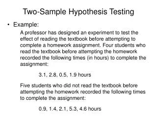
4. Example Suppose from a large class, we sample 4 grades: 64, 66, 89, 77. From another large class, we sample 3 grades: 56, 71, 53. We assume that the class grades are normally distributed, and that the population variances for the two classes are both 96.Test at the 5% level

5. As we’ve found before, the Z-values for a two tailed 5% test are 1.96 and -1.96, as indicated below. .475 .475 crit. reg. crit. reg. acceptance region .025 .025 Z -1.96 0 1.96 Since our Z-statistic, 1.87, is in the acceptance region, we accept H0: 1- 2= 0, concluding that the population means are equal.

6. What do you do if you don’t know the population variances in this formula? Replace the population variances with the sample variances and the Z distribution with the t distribution. The number of degrees of freedom is the integer part of this very messy formula:

7. Example Consider the same example as the last one but without the information on the population variances. Again test at the 5% level We need to determine the sample means and sample variances. As before, the sample means are 74 and 60.

8. So we subtract the sample mean from each of the grades.

9. Then we square those differences and add them up.

10. Then we divide that sum by n-1 to get the sample variance.

11. 0.95 0.025 0.025 -2.7764 0 2.7764 t4 What are the dof & critical t value? Since we have: our very messy dof formula yields So the degrees of freedom is the integer part of 4.86 or 4. For a 5% two-tailed test & 4 dof, the t value is 2.7764 .

12. 0.95 0.025 0.025 -2.7764 0 2.7764 t4 Next we need to compute our test statistic. Since our t-value, 1.748, is in the acceptance region, we accept H0: 1 = 2

13. Sometimes we don’t know the population variances, but we believe that they are equal. So we need to compute an estimate of the common variance, which we do by pooling our information from the two samples. We denote the pooled sample variance by sp2. sp2 is a weighted average of the two sample variances, with more weight put on the sample variance that was based on the larger sample. If the two samples are the same size, sp2 is just the sum of the two sample variances, divided by two. In general,

14. Let’s return for a moment to the statistic that we used to compare population means when the population variances were known. Then we can factor out the 2 and replace the 2 by sp2and the Z by t. The number of degrees of freedom is n1 + n2 -2.

15. crit. reg. crit. reg. Acceptance region .025 .025 0 -2.571 2.571 t5 Let’s do the previous example again, but this time assume that the unknown population variances are believed to be equal. We had: The number of degrees of freedom is n1 + n2 -2, and we are doing a 2-tailed test at the 5% level. Since our t-statistic 1.70 is in the acceptance region, we accept H0: 1 = 2.

16. In the previous three hypothesis tests, we tested whether 2 populations has the same mean, when we had 2 independent samples. • We can’t use those tests, however, if the 2 samples are not independent. • For example, suppose you are looking at the weights of people, before and after a fitness program. • Since the weights are for the same group of people, the before and after weights are not independent of each other. • In this type of situation, we can use a hypothesis test based on matched-pairs samples.

17. The hypotheses are The test statistic is

18. Example

19. First we calculate the weight differences.

20. Then we add up the differences and determine the mean.

21. Next we need to calculate the sample standard deviation for the weight differences. The sample standard deviation is

22. We subtract the mean difference from each of the D values.

23. We square the values in that column, and add up the squares.

24. Then since we divide by n-1 = 4, and take the square root.

25. Next we assemble our statistic.

26. crit. reg. crit. reg. Acceptance region .025 .025 0 -2.776 2.776 t4 Since we had 5 people and 5 pairs of weights, n=5, and the number of degrees of freedom is n-1 = 4. We’re doing a 2-tailed t-test at the 5% level, so the critical region looks like this: Since our t-statistic, -2.35, is in the acceptance region, we accept the null hypothesis that the program would cause no average weight change for the population as a whole.

27. Hypothesis tests on the difference between 2 population proportions, using independent samples If you look at the statistics we have used in our hypothesis tests, you will notice that they have a common form: In our hypothesis tests on the difference between 2 population proportions, we are going to use that same form.

28. We still need to determine the standard deviation, or an estimate of the standard deviation, of our point estimate.

30. Assembling the pieces, we have

31. Suppose the proportions of Democrats in samples of 100 and 225 from 2 states are 33% and 20%. Test at the 5% level the hypothesis that the proportion of Democrats in the populations of the 2 states are equal.

32. We’re doing a 2-tailed Z-test at the 5% level, so the critical region looks like this: crit. reg. crit. reg. Acceptance region .025 .025 0 -1.96 1.96 Z Since our Z-statistic, 2.53, is in the critical region, we reject the null hypothesis and accept the alternative that the proportions of Democrats in the 2 states are different.

33. Sometimes you want to test whether two independent samples have the same variance. If the populations are normally distributed, we can use the F-statistic to perform the test.

34. The F-statistic is This F-statistic has n1-1 degrees of freedom for the numerator, and n2-1 degrees of freedom for the denominator.

35. The distribution of our F-statistic, with the tail for the critical region looks like this: f(F) acceptance region critical region

36. Two-sided versus one-sided tests for equality of variance While you are always using the upper tail of the F-test on tests of equality of variance, the size of the critical region you sketch varies with whether you have a two-sided or a one-sided test. Let’s see why this is true.

37. While, for our samples, the sample variance from the first group was greater, our alternative hypothesis indicates that we think that the population variance could have been larger or smaller for the first population: Our sketch of the critical region is based on the situation in which the variance is greater for the first group, but we admit that, if we had information for the entire population, we might find that the situation is reversed. So there is an implicit second sketch of an F-statistic in which the sample variance of the second group is in the numerator. Thus, for each of the sketches, the sketch we draw and the implicit sketch, the area of the critical region is α/2, half of the test level α. So, for example, if you are doing a two-sided test at the 5% level, your sketch will show a tail area of 0.025.

38. What if we are performing a one-sided test? Now we are looking at a situation in which the sample variance is again larger for the first group. This time however, we want to know if, in fact, the population variance is really larger for the first group. So we have the one-sided alternative shown above. Keep in mind that, as usual with one-sided tests, the null hypothesis is the devil’s advocate view. Here the devil’s advocate is saying: nah, the population variance for the first group isn’t really any larger than for the second group. For a one-sided test with level α, your critical region will have area α. For example, if you are performing a one-sided test at the 5% level, the critical region will have area 0.05.

39. Example: You are looking at test results for two groups of students. There are 25 students in the first group, for which you have calculated the sample variance to be 15. There are 30 students in the second group, for which you have calculated the sample variance to be 10. Test at the 10% level whether the populations variances are the same. There are 25-1 = 24 degrees of freedom in the numerator and 30-1=29 degrees of freedom in the denominator. This is a two-sided test, so the critical region has area 0.05. f(F) Because 1.5 is in the acceptance region, you cannot reject the null hypothesis and you conclude that the variances of the two populations are the same. acceptance region critical region 0.05 1.90 F24, 29

40. In the two sections we have just completed, we did 9 different types of hypothesis tests. • population mean - 1 sample - known population variance • population mean - 1 sample - unknown population variance • population proportion - 1 sample • difference in population means - 2 independent samples - known population variances • difference in population means - 2 independent samples - unknown population variances • difference in population means - 2 independent samples - unknown population variances that are believed to be equal • difference in population means - 2 dependent samples • difference in population proportions - 2 independent samples • Difference in population variances - 2 independent samples • The statistics for these tests are compiled on a summary sheet which is available at my web site.