Download
1 / 33
330 likes | 522 Vues
Dynamic Set ADT Balanced Trees. Gerda Kamberova Department of Computer Science Hofstra University. Overview. Dynamic set ADT implemented with BST Balanced search trees AVL trees Definition Dynamic set implementation Complexity of the operation Red-Black trees Definition

E N D
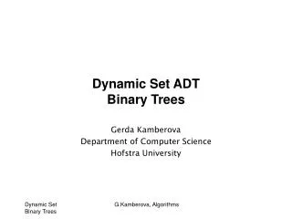
Dynamic Set ADTBalanced Trees Gerda Kamberova Department of Computer Science Hofstra University G.Kamberova, Algorithms
Overview • Dynamic set ADT implemented with BST • Balanced search trees • AVL trees • Definition • Dynamic set implementation • Complexity of the operation • Red-Black trees • Definition • Dynamic set implementation • Complexity of the operation G.Kamberova, Algorithms
Balanced BSTs • AVL Trees] (Adelson-Velskii and Landis, 1963). • Guaranteed worst-case • Red-Black Trees (Bayer, 1972). • Guaranteed worst- case • Superior to AVL trees in amortized sense (running time on a sequence of set operations). • Rotations are used to balance the AVL and RB trees. • Balancing is achieved by applying one or more times LR and/or RL basic rotations. • The rotations do not destroy BST property of the subtree on which they are performed. G.Kamberova, Algorithms
Basic Single Rotations Rotate left Rotate right p p v v Ta Tc LtoR Tb Tc Ta Tb RtoL G.Kamberova, Algorithms
AVL Trees • An AVL tree is a BST with • AVL property: the heights of the left and the right subtrees of any vertex differ at most by 1 • The height of an AVL tree containing n vertices is v Tl Tr h, h-1, or h+1 h G.Kamberova, Algorithms
AVL tree vertices • As with BST nodes contain key, data and pointers to parent, left and right children (the latter need to keep track of the link structure) • In addition, they have a field, called balance. • For a vertex v, the balance is the difference between the heights of the right and left subtree balance(v)=height(right(v)) - height(left(v)) • For every vertex v in an AVL tree, balance(v) is -1, 0, or 1 • If the balance of a vertex is different than 0,1,-1, the tree is not an AVL tree. G.Kamberova, Algorithms
Dynamic Set ADT with AVL trees • The search is a search on a BST • thus time complexity is O(h) • Height of any AVLT with n vertices is log n • Worst-case complexity is • Same thing true for min, max, predecessor, successor • Insert and Delete • may destroy the balance, thus the must be rebalanced using single or double rotations G.Kamberova, Algorithms
AVLT Insert • Insert as in BST, new nodes are inserted as leaves, this takes O(log n) • Retrace back the path from the new node to the root updating balances. This takes O(log n) • If a vertex x is encountered, balance(x)=2, adjust the tree rooted at the vertex by applying rotations so the balance becomes 0, -1 or 1. • Rebalance by a single or a double rotation • The single rotation pattern is given on figure 11.5 in the AVLT handout. • The double rotation pattern is given on figure 11.6 in the AVLT handout • Simplification: • The first vertex during the retrace whose balance was 1 prior the BST insert is the only vertex that can possibly get a new balance of 2. We call it potential pivot. • Only if the balance of the pivot becomes 2 after BST insert, the single or double rotation has to be performed only on the subtree rooted in the potential pivot, and this will rebalance the whole AVLT. • AVLT insert is O(log n) G.Kamberova, Algorithms
Single left-rotation (RtoL) pattern application +1 +2 0 +1 h+2 BST insert Ta Ta h h Tb Tc Tb Tc h h h h+1 0 0 Tc h+1 Tb h+1 Ta G.Kamberova, Algorithms
Double right-left-rotation (LtoR followed by RtoL) +2 +1 -1 0 A A 0 +1 D h D B C B C h-1 +2 +2 -1 0 A 0 B A B C D C D G.Kamberova, Algorithms
AVLT Delete • Perform delete on BST. This takes O(log n). • This could actually delete the predecessor or the successor vertex of the original vertex that had to be deleted • Retrace back the path from the parent of the actually deleted vertex to the root updating balances. • If a vertex with balance 2 found, adjust by rotations. • More then one rebalancing may be needed. • Since the total number of rebalances is bounded by the length of the path, the total number of rebalancing steps is O(log n) • Simplification: • If the balance of the parent of the deleted vertex changed to 1 , the height of the subtree rooted at the parent is the same, and the algorithm may terminate (Figure, 11.7). • In case the parent's balance went from 1 to 0, a rebalance may or may not be necessary (Figure 11.8). • AVLT delete is total O(log n). G.Kamberova, Algorithms
Red-Black Trees: augmenting the BST • RBT is an augmented BST that satisfies RBT property. • The augmented tree is defined as follows • External leaves are added to all null pointers. • This creates an augmented BST by adding n+1 leaves to the n vertex BST. • The external leaves are used only for the analysis, in practice it is not necessary to allocate memory for them. G.Kamberova, Algorithms
BST: example L E T J N V x G.Kamberova, Algorithms
Augmented BST: example L E T J N V x G.Kamberova, Algorithms
Red-Black Trees: Definition • A Red-Black three is an augmented BST in which every vertex is colored red or black in such a way that the RBT property is satisfied: • Black rule (BR): every leaf is black • Red rule (RR): if a vertex is red, its children are black • Path rule (PR): every path from the root to a leaf contains the same number of black vertices. • The path rule is satisfied for any vertex in RBT. Thus it makes sense to define black-height of a vertexbh(v) of v • bh(v) is the number of black nodes on the path from v to a leaf (but excluding v) G.Kamberova, Algorithms
RBT: example 2 L 1 2 E T 1 1 1 J N V 1 x • BR: every leaf is black • RR: if a vertex is red, its children are black • PR: every path from the root to a leaf contains the same number of black vertices • bh(v) is the number of black nodes on the path from v to a leaf (count the leaf , do not • count v) G.Kamberova, Algorithms
Red-Black Trees: tree height • What bound is the RBT property putting on the height of the three? • The height of RBT with n internal vertices is <= 2log(n+1), since • For any v, the subtree rooted in v contains at least vertices. Proof: by induction on the black-height, bh(v) 2. From RR, at least half of the vertices on any path from the root to a leaf must be black, so Since 2log(n+1)<=2log(2n)=2log(n)+2log(2), we have h<=2log(n) + Const, thus h = O(log n) G.Kamberova, Algorithms
RBT vertices • As with BST nodes contain key, data, and pointers to parent, left and right children (the latter need to keep track of the link structure) • In addition, a vertex has a field color (1 bit is enough to store it) • The color is used to compute the black-height and to check the RBT property G.Kamberova, Algorithms
Dynamic Set ADT with RB trees • Search • Perform search on BST. Since the height is O(log n), the search on RBT is O(log n) • Min, Max, Predecessor, Successor similarly are O(log n) • Insert and Delete may destroy the RBT property, thus to recover the RBT property, the tree has to be adjusted by recoloring and/or rotations G.Kamberova, Algorithms
RBT Insert • Perform insert on BST • Nodes inserted as leaves • The tree height is O(log n), thus this takes O(log n) • For the purpose of the analysis, think that instead of inserting a single node in BST, insert a subtree consisting of a red root (the vertex to be inserted), and two black children (with no data). • The BST insert will replace an external leaf in the augmented tree by a new subtree consisting of red root and two black children. • This insertion procedure preservesBR and PR rules, but may violate RR G.Kamberova, Algorithms
RBT: example, insert G 2 L 1 2 E T 1 1 1 J N V 1 x G G.Kamberova, Algorithms
Ex: The tree after BST inserted G 2 L 1 2 E T 1 1 1 J N V 1 G x BST insert violated RR G.Kamberova, Algorithms
RBT Insert • Recover the RBT property. • Let v be is the new insertion in the RBT T • v is red • Denote: p is parent of v, g = grand parent of v, u = uncle of v (u and p descend from g) • Ifv is the root, the new tree is RBT, done • If p is black, the new tree is RBT, done • If p is red , then recover RR by recoloring and/or rotations • 3.1 If p is the root make v black, done • 3.2 Otherwise, p is not the root: • Since p is red, g must be black (by RR). • Since T is augmented BST u exists • The color of u determines the method by which the RR will be recovered g p u v G.Kamberova, Algorithms
RBT Insert: cont 3.1 • Recover the RBT property. • 3.2, p is red, v is red, g is black, color of u will determine the method by which to recover RBT • If u is red, recolor: • If, g's parent is black, recolor as follows g red, p black, u black; done. • If g’s parent is red, • recolor again g red, p black, u black ; • now the problem that we had with the coloring of v and p (both red) is moved up at g and g’s parent (now these two are both red after the recoloring). • recursively apply the recoloring algorithm to (g, g’s parent) • In the worst case the recoloring will propagate all the way back to the root, O(log n) g p u RR violated v G.Kamberova, Algorithms
RBT Insert: cont 3.1 • Recover the RBT property. • 3.2, p is red, v is red, g is black, color of u will determine the method by which to recover RBT • If u is red, recolor: • If, g's parent is black, recolor as follows g red, p black, u black; done. • If g’s parent is red, • recolor again g red, p black, u black ; • now the problem that we had with the coloring of v and p (both red) is moved up at g and g’s parent (now these two are both red after the recoloring). • recursively apply the recoloring algorithm to (g, g’s parent) • In the worst case the recoloring will propagate all the way back to the root, O(log n) g p u v G.Kamberova, Algorithms
RBT Insert: cont 3.1 • Recover the RBT property. • 3.2, p is red, v is red, g is black, color of u will determine the method by which to recover RBT • If u is red, recolor: • If, g's parent is black, recolor as follows g red, p black, u black; done. • If g’s parent is red, • recolor again g red, p black, u black ; • now the problem that we had with the coloring of v and p (both red) is moved up at g and g’s parent. • recursively apply the recoloring algorithm to (g, g’s parent) • In the worst case the recoloring will propagate all the way back to the root g p u v G.Kamberova, Algorithms
RBT Insert: cont • Recover the RBT property. • 3.2 v is red, p is red, g is black, color of u will determine the method by which to recover RBT • If u is black • If v is left child of left parent (or right of right parent) • single LR (or RL)rotation at g (left-left shown in picture) • Recoloring • In the recoloring the root of the subtree ends up black, done. g p p u v v g u G.Kamberova, Algorithms
RBT Insert: cont • Recover the RBT property. • 3.2 v is red, p is red, g is black, color of u will determine the method by which to recover RBT • If u is black • If v is right child of left parent (or left of right parent) • RL (or LR) rotation at p • LR (or RL) rotation at g • Recoloring • In the recoloring the root of the subtree ends up black, done. g v p u g p g u v v u p G.Kamberova, Algorithms
RBT Insert complexity • BST insert is O(log n) • Each rotation/recoloring takes • In the worst case, recoloring/rotations may propagate to the root of the tree, and since the height is O(log n), the worst case time complexity of recovering RBT property is O(log n)* which is still O(log n) • Thus RVLT Insert is O(log n) G.Kamberova, Algorithms
RBT: example, insert G 2 L 1 2 E T 1 1 1 J N V 1 x G G.Kamberova, Algorithms
Ex: The tree after BST insert(G) L g E T p J N V u v G x p , g, u, v is left child of right parent G.Kamberova, Algorithms
Ex: The tree after BST insert(G) L g E T v G N V p J x u p , g, u, v was left child of right parent G.Kamberova, Algorithms
Ex: The tree after BST insert(G) L T G J N V E x p , g, u, v was left child of right parent G.Kamberova, Algorithms